Linealización de sistemas no lineales
IE3041 - Sistemas de Control 2

Un mundo no lineal

Clasificar los sistemas en lineales y no lineales es como clasificar los objetos en el universo como bananos y no bananos
- Desconocido
¿Qué podemos hacer al respecto?
\begin{cases} \dot{\mathbf{x}}=\mathbf{f}\left(\mathbf{x},\mathbf{u}\right) \\
\mathbf{y}=\mathbf{h}\left(\mathbf{x},\mathbf{u}\right) \\
\mathbf{x}(t_0)=\mathbf{x}_0 \end{cases}
¿Qué podemos hacer al respecto?
\begin{cases} \dot{\mathbf{x}}=\mathbf{A}\mathbf{x}+\mathbf{B}\mathbf{u} \\
\mathbf{y}=\mathbf{C}\mathbf{x}+\mathbf{D}\mathbf{u} \\
\mathbf{x}(t_0)=\mathbf{x}_0 \end{cases}
\begin{cases} \dot{\mathbf{x}}=\mathbf{f}\left(\mathbf{x},\mathbf{u}\right) \\
\mathbf{y}=\mathbf{h}\left(\mathbf{x},\mathbf{u}\right) \\
\mathbf{x}(t_0)=\mathbf{x}_0 \end{cases}
Linealización
¿Problema?
los sistemas LTI presentan un único comportamiento general en todo su espacio de estados:
convergencia, divergencia u oscilación
¿Problema?
los sistemas LTI presentan un único comportamiento general en todo su espacio de estados:
convergencia, divergencia u oscilación
NUNCA más de uno
ie3041_clase3_randlti2dpp¿Problema?
en contraste, los sistemas no lineales pueden presentar múltiples comportamientos en su espacio de estados.
ej: >> PendSim
los sistemas LTI presentan un único comportamiento general en todo su espacio de estados:
convergencia, divergencia u oscilación
NUNCA más de uno
ie3041_clase3_randlti2dpp¿Solución?
múltiples linealizaciones, una para cada tipo de comportamiento
¿Solución?
múltiples linealizaciones, una para cada tipo de comportamiento
punto fijo

linealización local alrededor de un
punto de equilibrio
Puntos de equilibrio
punto de equilibrio
\(\left(\mathbf{x}^*,\mathbf{u}^*\right)\)
el sistema deja de evolucionar
\(\dot{\mathbf{x}}=\mathbf{0}\)
\(\mathbf{f}\left(\mathbf{x}^*,\mathbf{u}^*\right)=\mathbf{0}\)
\boldsymbol\Rightarrow
si \(\mathbf{u}^*=\mathbf{0}\) el punto recibe el nombre de punto de equilibrio (natural)
Puntos de equilibrio
punto de equilibrio
\(\left(\mathbf{x}^*,\mathbf{u}^*\right)\)
el sistema deja de evolucionar
\(\dot{\mathbf{x}}=\mathbf{0}\)
\(\mathbf{f}\left(\mathbf{x}^*,\mathbf{u}^*\right)=\mathbf{0}\)
\boldsymbol\Rightarrow
si \(\mathbf{u}^*\ne\mathbf{0}\) entonces el punto cambia a \(\left(\mathbf{x}_{ss},\mathbf{u}_{ss}\right)\) y se llama equilibrio forzado o punto de operación
punto de operación
punto de operación
el caso de un punto de operación corresponde a un problema de regulación (referencia constante) en control clásico
Ejemplo: péndulo simple
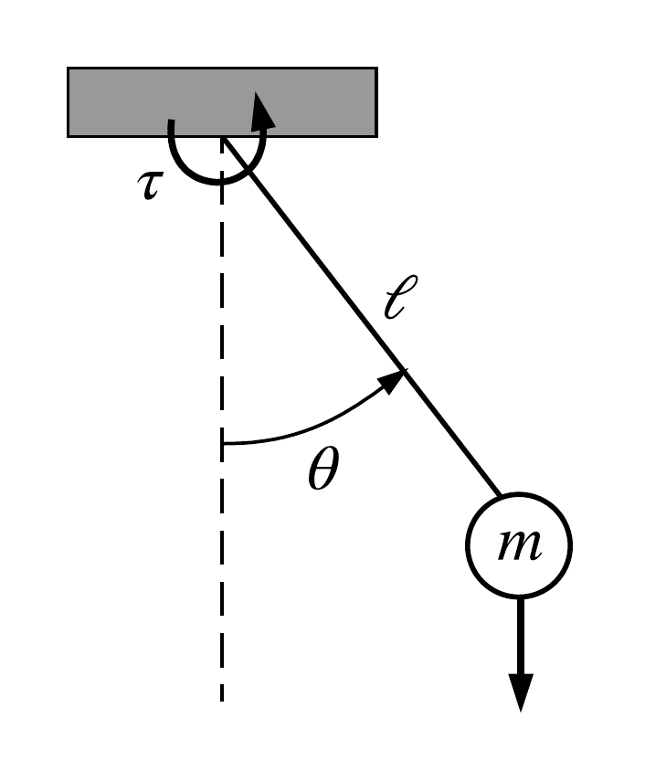
\dot{\mathbf{x}}=\mathbf{f}\left(\mathbf{x},u\right)=\begin{bmatrix} x_2 \\ -(g/\ell)\sin(x_1)+(1/m\ell^2)u\end{bmatrix}
Ejemplo: péndulo simple
\dot{\mathbf{x}}=\mathbf{f}\left(\mathbf{x},u\right)=\begin{bmatrix} x_2 \\ -(g/\ell)\sin(x_1)+(1/m\ell^2)u\end{bmatrix}
\mathbf{x}^*=\begin{bmatrix} x_1^* \\ x_2^* \end{bmatrix}=\begin{bmatrix} k\pi, \ k\in\mathbb{Z} \\ 0 \end{bmatrix}, \quad u^*=0
\mathbf{x}_{ss}=\begin{bmatrix} x_{1,ss} \\ x_{2,ss} \end{bmatrix}=\begin{bmatrix} \delta \\ 0 \end{bmatrix}, \quad u_{ss}=mg\ell\sin\delta
Encontrando puntos de equilibrio
punto de equilibrio
punto de operación
\mathbf{f}\left(\mathbf{x}^*, \mathbf{0}\right)=\mathbf{0}
\mathbf{f}\left(\mathbf{x}_{ss}, \mathbf{u}_{ss}\right)=\mathbf{0}
Encontrando puntos de equilibrio
punto de equilibrio
punto de operación
\mathbf{f}\left(\mathbf{x}^*, \mathbf{0}\right)=\mathbf{0}
\mathbf{f}\left(\mathbf{x}_{ss}, \mathbf{u}_{ss}\right)=\mathbf{0}
requerimientos de control
Encontrando puntos de equilibrio
punto de equilibrio
punto de operación
\mathbf{f}\left(\mathbf{x}^*, \mathbf{0}\right)=\mathbf{0}
\mathbf{f}\left(\mathbf{x}_{ss}, \mathbf{u}_{ss}\right)=\mathbf{0}
\mathbf{F}\left(\mathbf{z}\right)=\mathbf{0}
\mathbf{z}=\mathbf{x}^*
\mathbf{z}=\mathbf{u}_{ss}
sistema de ecuaciones algebraicas no lineales
requerimientos de control
difícil
(analíticamente)
Paréntesis: el método de Newton
\mathbf{F}\left(\mathbf{z}\right)=\mathbf{0}
\mathbf{z}_{i+1}=\mathbf{z}_i+\Delta\mathbf{z}
D \mathbf{F}\left(\mathbf{z}_i\right)\Delta\mathbf{z}=-\mathbf{F}\left(\mathbf{z}_i \right)
1)
2)
Paréntesis: el método de Newton
\mathbf{F}\left(\mathbf{z}\right)=\mathbf{0}
% Definición de la función no lineal
F = @(z) ... % o bien en un archivo de función aparte (ej. fun.m)

z0 = [...]; % aproximación inicial (initial guess)

% Se resuelve numéricamente el sistema
z_sol = fsolve(F, z0);

% Para las funciones aparte se manda el handle, es decir
z_sol = fsolve(@fun, z0);
Regresando a las linealizaciones locales
\mathbf{x}(t_0)=\mathbf{x}^*+\delta\mathbf{x}^*

\mathbf{x}(t)=\mathbf{x}^*+\delta\mathbf{x}(t)
\mathbf{u}(t)=\mathbf{u}^*+\delta\mathbf{u}(t)
\Rightarrow \dot{\delta\mathbf{x}}=\mathbf{f}\left(\mathbf{x}^*+\delta\mathbf{x}, \mathbf{u}^*+\delta\mathbf{u}\right)
\mathbf{x}(t_0)=\mathbf{x}^*+\delta\mathbf{x}^*
\mathbf{x}(t)=\mathbf{x}^*+\delta\mathbf{x}(t)
\mathbf{u}(t)=\mathbf{u}^*+\delta\mathbf{u}(t)
\Rightarrow \dot{\delta\mathbf{x}}=\mathbf{f}\left(\mathbf{x}^*+\delta\mathbf{x}, \mathbf{u}^*+\delta\mathbf{u}\right)
+ expansión por Series de Taylor ...
\begin{cases} \dot{\mathbf{z}}=\mathbf{A}\mathbf{z}+\mathbf{B}\mathbf{v} \\
\mathbf{w}=\mathbf{C}\mathbf{z}+\mathbf{D}\mathbf{v} \\
\mathbf{z}(t_0)=\mathbf{z}_0 \end{cases}
\begin{cases} \dot{\mathbf{z}}=\mathbf{A}\mathbf{z}+\mathbf{B}\mathbf{v} \\
\mathbf{w}=\mathbf{C}\mathbf{z}+\mathbf{D}\mathbf{v} \\
\mathbf{z}(t_0)=\mathbf{z}_0=\delta\mathbf{x}^* \end{cases}
\mathbf{z}=\delta\mathbf{x}=\mathbf{x}-\mathbf{x}^*
\mathbf{v}=\delta\mathbf{u}=\mathbf{u}-\mathbf{u}^*
\mathbf{w}=\delta\mathbf{y}=\mathbf{y}-\mathbf{h}\left(\mathbf{x}^*,\mathbf{u}^*\right)
\begin{cases} \dot{\mathbf{z}}=\mathbf{A}\mathbf{z}+\mathbf{B}\mathbf{v} \\
\mathbf{w}=\mathbf{C}\mathbf{z}+\mathbf{D}\mathbf{v} \\
\mathbf{z}(t_0)=\mathbf{z}_0=\delta\mathbf{x}^* \end{cases}
\mathbf{A}=\dfrac{\partial \mathbf{f}\left(\mathbf{x}^*,\mathbf{u}^*\right)}{\partial \mathbf{x}}=
\begin{bmatrix} \frac{\partial f_1\left(\mathbf{x}^*,\mathbf{u}^*\right)}{\partial x_1} & \cdots & \frac{\partial f_1\left(\mathbf{x}^*,\mathbf{u}^*\right)}{\partial x_n} \\
\vdots & \ddots & \vdots \\
\frac{\partial f_n\left(\mathbf{x}^*,\mathbf{u}^*\right)}{\partial x_1} & \cdots & \frac{\partial f_n\left(\mathbf{x}^*,\mathbf{u}^*\right)}{\partial x_n} \end{bmatrix}
\begin{cases} \dot{\mathbf{z}}=\mathbf{A}\mathbf{z}+\mathbf{B}\mathbf{v} \\
\mathbf{w}=\mathbf{C}\mathbf{z}+\mathbf{D}\mathbf{v} \\
\mathbf{z}(t_0)=\mathbf{z}_0=\delta\mathbf{x}^* \end{cases}
\mathbf{B}=\dfrac{\partial \mathbf{f}\left(\mathbf{x}^*,\mathbf{u}^*\right)}{\partial \mathbf{u}}=
\begin{bmatrix} \frac{\partial f_1\left(\mathbf{x}^*,\mathbf{u}^*\right)}{\partial u_1} & \cdots & \frac{\partial f_1\left(\mathbf{x}^*,\mathbf{u}^*\right)}{\partial u_m} \\
\vdots & \ddots & \vdots \\
\frac{\partial f_n\left(\mathbf{x}^*,\mathbf{u}^*\right)}{\partial u_1} & \cdots & \frac{\partial f_n\left(\mathbf{x}^*,\mathbf{u}^*\right)}{\partial u_m} \end{bmatrix}
\begin{cases} \dot{\mathbf{z}}=\mathbf{A}\mathbf{z}+\mathbf{B}\mathbf{v} \\
\mathbf{w}=\mathbf{C}\mathbf{z}+\mathbf{D}\mathbf{v} \\
\mathbf{z}(t_0)=\mathbf{z}_0=\delta\mathbf{x}^* \end{cases}
\mathbf{C}=\dfrac{\partial \mathbf{h}\left(\mathbf{x}^*,\mathbf{u}^*\right)}{\partial \mathbf{x}}=
\begin{bmatrix} \frac{\partial h_1\left(\mathbf{x}^*,\mathbf{u}^*\right)}{\partial x_1} & \cdots & \frac{\partial h_1\left(\mathbf{x}^*,\mathbf{u}^*\right)}{\partial x_n} \\
\vdots & \ddots & \vdots \\
\frac{\partial h_p\left(\mathbf{x}^*,\mathbf{u}^*\right)}{\partial x_1} & \cdots & \frac{\partial h_p\left(\mathbf{x}^*,\mathbf{u}^*\right)}{\partial x_n} \end{bmatrix}
\begin{cases} \dot{\mathbf{z}}=\mathbf{A}\mathbf{z}+\mathbf{B}\mathbf{v} \\
\mathbf{w}=\mathbf{C}\mathbf{z}+\mathbf{D}\mathbf{v} \\
\mathbf{z}(t_0)=\mathbf{z}_0=\delta\mathbf{x}^* \end{cases}
\mathbf{D}=\dfrac{\partial \mathbf{h}\left(\mathbf{x}^*,\mathbf{u}^*\right)}{\partial \mathbf{u}}=
\begin{bmatrix} \frac{\partial h_1\left(\mathbf{x}^*,\mathbf{u}^*\right)}{\partial u_1} & \cdots & \frac{\partial h_1\left(\mathbf{x}^*,\mathbf{u}^*\right)}{\partial u_m} \\
\vdots & \ddots & \vdots \\
\frac{\partial h_p\left(\mathbf{x}^*,\mathbf{u}^*\right)}{\partial u_1} & \cdots & \frac{\partial h_p\left(\mathbf{x}^*,\mathbf{u}^*\right)}{\partial u_m} \end{bmatrix}
basta hacer el cambio \(\left(\mathbf{x}^*,\mathbf{u}^*\right)=\left(\mathbf{x}_{ss},\mathbf{u}_{ss}\right)\) para el caso de un punto de operación
Ejemplo: péndulo simple
\dot{\mathbf{x}}=\mathbf{f}\left(\mathbf{x},u\right)=\begin{bmatrix} x_2 \\ -(g/\ell)\sin(x_1)+(1/m\ell^2)u\end{bmatrix}
y=h\left(\mathbf{x},u\right)=\arctan(x_1)
Ejemplo: péndulo simple
\dot{\mathbf{x}}=\mathbf{f}\left(\mathbf{x},u\right)=\begin{bmatrix} x_2 \\ -(g/\ell)\sin(x_1)+(1/m\ell^2)u\end{bmatrix}
y=h\left(\mathbf{x},u\right)=\arctan(x_1)
\mathbf{x}^*=\begin{bmatrix} x_1^* \\ x_2^* \end{bmatrix}=\begin{bmatrix} 0 \\ 0 \end{bmatrix}, \ u^*=0
\dot{\mathbf{z}}=\begin{bmatrix} 0 & 1 \\ -g/\ell & 0 \end{bmatrix}\mathbf{z}+\begin{bmatrix} 0 \\ 1/m\ell^2 \end{bmatrix}v
w = \begin{bmatrix} 1 & 0 \end{bmatrix}\mathbf{z}
Ejemplo: péndulo simple
\dot{\mathbf{x}}=\mathbf{f}\left(\mathbf{x},u\right)=\begin{bmatrix} x_2 \\ -(g/\ell)\sin(x_1)+(1/m\ell^2)u\end{bmatrix}
y=h\left(\mathbf{x},u\right)=\arctan(x_1)
ie3041_clase3_pendlin(xss, delta)>> ie3041_clase3_linealizacion.mlx
¿Problema?
similar al caso de buscar puntos de equilibrio u operación, la linealización es difícil (analíticamente)
¿Problema?
similar al caso de buscar puntos de equilibrio u operación, la linealización es difícil (analíticamente)
¿Solución?
Linealización numérica
\dfrac{df(x)}{dx} \approx \dfrac{f(x+\delta x)-f(x)}{\delta x}
diferencias finitas
\dfrac{df(x)}{dx} \approx \dfrac{f(x+\delta x)-f(x)}{\delta x}
diferencias finitas
\dfrac{\partial \mathbf{f}\left(\mathbf{x},\mathbf{u}\right)}{\partial x_j} \approx
\dfrac{\mathbf{f}\left(\mathbf{x}+\delta x\mathbf{e}_j,\mathbf{u}\right)-\mathbf{f}\left(\mathbf{x},\mathbf{u}\right)}{\delta x}
for \(j=1,2,\cdots,n\)
ej: \(n=3, \ \mathbf{e}_2=\begin{bmatrix} 0 & 1 & 0 \end{bmatrix}^\top\)
lo más pequeño posible*
se hace un proceso similar para obtener el resto de jacobianos
resultado:
loclin_fast con forward finite difference
(menos evaluaciones)
loclin_best con central finite difference
(más exacto pero ligeramente lento)
>> ie3041_clase3_linealizacion.mlx
¿Qué ventajas nos trae esto?
\begin{cases} \dot{\mathbf{x}}=\mathbf{f}\left(\mathbf{x},\mathbf{u}\right) \\
\mathbf{y}=\mathbf{h}\left(\mathbf{x},\mathbf{u}\right) \\
\mathbf{x}(t_0)=\mathbf{x}_0 \end{cases}
pueden evaluarse | obtenerse mediante simuladores o identificarse (aprenderse) sin necesidad de efectuar modelado
Ejemplo: péndulo doble
\ell_1
\ell_2
m_1
m_2
q_1
q_2
Ejemplo: péndulo doble
\ell_1
\ell_2
m_1
m_2
q_1
q_2
¿Dinámica y jacobianos?
\((m_1+m_2)\ell_1^2\ddot{q}_1+m_2\ell_2^2\left(\ddot{q}_1+\ddot{q}_2\right)+m_2\ell_1\ell_2\left(2\ddot{q}_1+\ddot{q}_2\right)\cos(q_2)-m_2\ell_1\ell_2\left(2\dot{q}_1+\dot{q}_2\right)\dot{q}_2\sin(q_2)+(m_1+m_2)\ell_1g\sin(q_1)+m_2g\ell_2\sin(q_1+q_2)=\tau_1\)
\( m_2\ell_2^2\left(\ddot{q}_1+\ddot{q}_2\right)+m_2\ell_1\ell_2\ddot{q}_1\cos(q_2)+m_2\ell_1\ell_2\dot{q}_1^2\sin(q_2)+m_2g\ell_2\sin(q_1+q_2)=\tau_2\)
Ejemplo: péndulo doble
\ell_1
\ell_2
m_1
m_2
q_1
q_2

(u otra herramienta de simulación)
+ linealización numérica
>> ie3041_clase3_dblpend
¿Más allá de puntos de equilibrio y operación?

linealización local alrededor de una órbita o trayectoria
Trayectorias nominales (soluciones)
\(\left(\mathbf{x}^*(t), \mathbf{u}^*(t)\right)\) es una solución o trayectoria nominal si
\dot{\mathbf{x}}^*(t)=\mathbf{f}\left(\mathbf{x}^*(t),\mathbf{u}^*(t)\right)
Trayectorias nominales (soluciones)
\(\left(\mathbf{x}^*(t), \mathbf{u}^*(t)\right)\) es una solución o trayectoria nominal si
\dot{\mathbf{x}}^*(t)=\mathbf{f}\left(\mathbf{x}^*(t),\mathbf{u}^*(t)\right)
es decir, son soluciones particulares de la EDO o bien el resultado de una simulación
\begin{cases} \dot{\mathbf{z}}=\mathbf{A}(t)\mathbf{z}+\mathbf{B}(t)\mathbf{v} \\
\mathbf{w}=\mathbf{C}(t)\mathbf{z}+\mathbf{D}(t)\mathbf{v} \\
\mathbf{z}(t_0)=\mathbf{z}_0=\delta\mathbf{x}_d \end{cases}
\mathbf{z}(t)=\delta\mathbf{x}(t)=\mathbf{x}(t)-\mathbf{x}_d(t),
\mathbf{v}(t)=\delta\mathbf{u}(t)=\mathbf{u}(t)-\mathbf{u}_d(t),
\mathbf{w}(t)=\delta\mathbf{y}(t)=\mathbf{y}(t)-\mathbf{h}\left(\mathbf{x}_d(t),\mathbf{u}_d(t)\right)
el punto de linealización cambia (trayectoria)
\(\Rightarrow\) sistema LTV
las desviaciones son ahora con respecto de una trayectoria deseada \(\left(\mathbf{x}_d(t),\mathbf{u}_d(t)\right)\)
el punto de linealización cambia (trayectoria)
\(\Rightarrow\) sistema LTV
las desviaciones son ahora con respecto de una trayectoria deseada \(\left(\mathbf{x}_d(t),\mathbf{u}_d(t)\right)\)
equivalente a un problema de rastreo de referencia en control clásico
el punto de linealización cambia (trayectoria)
\(\Rightarrow\) sistema LTV
las desviaciones son ahora con respecto de una trayectoria deseada \(\left(\mathbf{x}_d(t),\mathbf{u}_d(t)\right)\)
equivalente a un problema de rastreo de referencia en control clásico
>> ie3041_clase3_linealizacion.mlx
Trayectorias deseadas

Trayectorias deseadas
\mathbf{x} \in \mathbb{R}^{50}
\mathbf{u} \in \mathbb{R}^{25}
Trayectorias deseadas
\mathbf{x} \in \mathbb{R}^{50}
\mathbf{u} \in \mathbb{R}^{25}
\left(\mathbf{x}_d(t),\mathbf{u}_d(t)\right)
Trayectorias deseadas
\mathbf{x} \in \mathbb{R}^{50}
\mathbf{u} \in \mathbb{R}^{25}
\left(\mathbf{x}_d(t),\mathbf{u}_d(t)\right)
encontrar trayectorias deseadas NO es trivial
\(\Rightarrow\) optimización de trayectorias
(más adelante en el curso...)
¿Linealizaciones que no sean locales?
Dos ideas prevalentes
¿Linealizaciones que no sean locales?
Linealización por retroalimentación
Idea: usar control para "eliminar" las no linealidades
Linealización por retroalimentación
\dot{\mathbf{x}}=\mathbf{f}\left(\mathbf{x},\mathbf{u}\right)=\mathbf{f}\left(\mathbf{x}\right)+\mathbf{G}\left(\mathbf{x}\right)\mathbf{u}
para algunos sistemas de control afines
Linealización por retroalimentación
\dot{\mathbf{x}}=\mathbf{f}\left(\mathbf{x},\mathbf{u}\right)=\mathbf{f}\left(\mathbf{x}\right)+\mathbf{G}\left(\mathbf{x}\right)\mathbf{u}
"puede emplearse" la ley de retroalimentación
para algunos sistemas de control afines
\mathbf{u}\approx \mathbf{G}^{-1}\left(\mathbf{x}\right)\left[\mathbf{v}-\mathbf{f}\left(\mathbf{x}\right)\right]
Linealización por retroalimentación
para "cancelar la dinámica" del sistema tal que
\dot{\mathbf{x}} \approx \mathbf{v}
Linealización por retroalimentación
o bien obtener un sistema LTI
para "cancelar la dinámica" del sistema tal que
\dot{\mathbf{z}}= \mathbf{A}\mathbf{z}+\mathbf{B}\mathbf{v}
\dot{\mathbf{x}} \approx \mathbf{v}
bajo el difeomorfismo \(\mathbf{z}=T\left(\mathbf{x}\right)\)
Ejemplo: péndulo simple
\dot{\mathbf{x}}=\mathbf{f}\left(\mathbf{x},u\right)=\begin{bmatrix} x_2 \\ -(g/\ell)\sin(x_1)+(1/m\ell^2)u\end{bmatrix}
Ejemplo: péndulo simple
\dot{\mathbf{x}}=\mathbf{f}\left(\mathbf{x},u\right)=\begin{bmatrix} x_2 \\ -(g/\ell)\sin(x_1)+(1/m\ell^2)u\end{bmatrix}
no linealidad,
debe emplearse \(u\) para eliminarla
Ejemplo: péndulo simple
\dot{\mathbf{x}}=\mathbf{f}\left(\mathbf{x},u\right)=\begin{bmatrix} x_2 \\ -(g/\ell)\sin(x_1)+(1/m\ell^2)u\end{bmatrix}
no linealidad,
debe emplearse \(u\) para eliminarla
u=m\ell^2\left[v+(g/\ell)\sin(x_1)\right]
\Rightarrow \dot{\mathbf{x}}=\begin{bmatrix} x_2 \\ v \end{bmatrix}
=\begin{bmatrix} 0 & 1 \\ 0 & 0 \end{bmatrix} \begin{bmatrix} x_1 \\ x_2 \end{bmatrix}+ \begin{bmatrix} 0 \\ 1 \end{bmatrix}v
¿Problemas con esta idea?
¿Cuándo funciona? (actuación)
¿Problemas con esta idea?
¿Qué tan caro es cancelar la dinámica? (eficiencia)
¿Cuándo funciona? (actuación)
¿Problemas con esta idea?
¿Qué tan caro es cancelar la dinámica? (eficiencia)
¿Qué tan bueno es el modelo del sistema como para que sepamos qué cancelar? (robustez)
¿Cuándo funciona? (actuación)
¿Problemas con esta idea?
a pesar de esto, figura como la herramienta fundamental detrás de muchos métodos de control no lineal
Teoría de Koopman
Idea: pueden "eliminarse" las no linealidades bajo una selección correcta de variables
Teoría de Koopman
Idea: pueden "eliminarse" las no linealidades bajo una selección correcta de variables
\mathbf{z}=\mathbf{g}\left(\mathbf{x}\right) \in \mathbb{R}^q, \quad q\ge n
observables
\(\approx\) salidas | mediciones
Teoría de Koopman
Idea: pueden "eliminarse" las no linealidades bajo una selección correcta de variables
\mathbf{z}=\mathbf{g}\left(\mathbf{x}\right) \in \mathbb{R}^q, \quad q\ge n
observables
\(\approx\) salidas | mediciones
NOTA: el planteamiento original de Koopman no considera entradas
Teoría de Koopman
conforme \(q\to\infty\), Koopman establece que
\dot{\mathbf{x}}=\mathbf{f}\left(\mathbf{x}\right) \ \to \ \dot{\mathbf{z}}=\boldsymbol{\mathcal{K}} \mathbf{z}
Teoría de Koopman
conforme \(q\to\infty\), Koopman establece que
\dot{\mathbf{x}}=\mathbf{f}\left(\mathbf{x}\right) \ \to \ \dot{\mathbf{z}}=\boldsymbol{\mathcal{K}} \mathbf{z}
es decir, todo sistema dinámico (no lineal) es lineal en un espacio suficientemente grande* de observables
Ejemplo básico
\dot{\mathbf{x}}=\mathbf{f}\left(\mathbf{x}\right)=\begin{bmatrix} \mu x_1 \\ \lambda\left(x_2-x_1^2\right) \end{bmatrix}
Ejemplo básico
\dot{\mathbf{x}}=\mathbf{f}\left(\mathbf{x}\right)=\begin{bmatrix} \mu x_1 \\ \lambda\left(x_2-x_1^2\right) \end{bmatrix}
\mathbf{z}=\begin{bmatrix} z_1 \\ z_2 \\ z_3 \end{bmatrix}=\begin{bmatrix} x_1 \\ x_2 \\ x_1^2 \end{bmatrix}
observables
Ejemplo básico
\dot{\mathbf{x}}=\mathbf{f}\left(\mathbf{x}\right)=\begin{bmatrix} \mu x_1 \\ \lambda\left(x_2-x_1^2\right) \end{bmatrix}
\Rightarrow \dot{\mathbf{z}}=\begin{bmatrix} \dot{z}_1 \\ \dot{z}_2 \\ \dot{z}_3 \end{bmatrix}
=\begin{bmatrix} \dot{x}_1=\mu z_1 \\ \dot{x}_2=\lambda(z_2-z_3) \\ 2x_1\dot{x}_1=2\mu x_1^2=2\mu z_3 \end{bmatrix}
=\begin{bmatrix} \mu & 0 & 0 \\ 0 & \lambda & -\lambda \\ 0 & 0 & 2\mu \end{bmatrix} \begin{bmatrix} z_1 \\ z_2 \\ z_3 \end{bmatrix}
\mathbf{z}=\begin{bmatrix} z_1 \\ z_2 \\ z_3 \end{bmatrix}=\begin{bmatrix} x_1 \\ x_2 \\ x_1^2 \end{bmatrix}
observables
Ejemplo: péndulo simple
\dot{\mathbf{x}}=\mathbf{f}\left(\mathbf{x},u\right)=\begin{bmatrix} x_2 \\ -(g/\ell)\sin(x_1)\end{bmatrix}
Ejemplo: péndulo simple
\dot{\mathbf{x}}=\mathbf{f}\left(\mathbf{x},u\right)=\begin{bmatrix} x_2 \\ -(g/\ell)\sin(x_1)\end{bmatrix}
\mathbf{z}=\begin{bmatrix} z_1 \\ z_2 \\ z_3 \\ \vdots \end{bmatrix}=\begin{bmatrix} x_1 \\ x_2 \\ \sin(x_1) \\ \vdots \end{bmatrix}
observables
Ejemplo: péndulo simple
\dot{\mathbf{x}}=\mathbf{f}\left(\mathbf{x},u\right)=\begin{bmatrix} x_2 \\ -(g/\ell)\sin(x_1)\end{bmatrix}
\Rightarrow \dot{\mathbf{z}}=\begin{bmatrix} \dot{z}_1 \\ \dot{z}_2 \\ \dot{z}_3 \\ \vdots \end{bmatrix}=\begin{bmatrix} z_2 \\ -(g/\ell) z_3 \\ \cos(x_1)x_2 \\ \vdots \end{bmatrix}
???
¿Problemas con esta idea?
¿Cuáles y cuántos observables?
¿Problemas con esta idea?
¿Qué ocurre con los múltiples comportamientos (puntos de equilibrio)?
¿Cuáles y cuántos observables?
¿Problemas con esta idea?
¿Qué ocurre con los múltiples comportamientos (puntos de equilibrio)?
Si casi nunca puede hacerse analíticamente, ¿Cómo se hace numéricamente?
¿Cuáles y cuántos observables?
¿Problemas con esta idea?
sin embargo, recientemente esta forma de análisis se ha vuelto clave en el área de data-driven dynamical systems
IE3041 - Lecture 3 (2025)
By Miguel Enrique Zea Arenales


