Estabilización de trayectorias
IE3041 - Sistemas de Control 2

¿Dónde estamos por el momento?
condición inicial \(\mathbf{x}_0\)
"meta" \(\mathbf{x}_{ss}\)
condición inicial \(\mathbf{x}_0\)
"meta" \(\mathbf{x}_{ss}\)
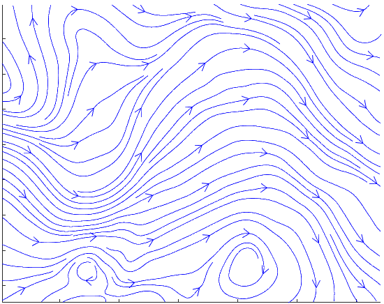
fuimos capaces de emplear colocación directa para encontrar la trayectoria óptima
esta, sin embargo, presenta un problema crítico
esta, sin embargo, presenta un problema crítico
un ligero cambio en la trayectoria causa un comportamiento completamente distinto
esta, sin embargo, presenta un problema crítico
un ligero cambio en la trayectoria causa un comportamiento completamente distinto
¿Por qué?
\mathbf{u}^\star \equiv \mathbf{u}\left(\mathbf{x}(t)\right)
lazo cerrado
\mathbf{u}^\star \equiv \mathbf{u}\left(\mathbf{x}(t)\right)
\mathbf{u}^\star \equiv \mathbf{u}(t)
lazo cerrado
lazo abierto
\mathbf{u}^\star \equiv \mathbf{u}(t)
lazo abierto
\mathbf{u}^\star \equiv \mathbf{u}\left(\mathbf{x}(t)\right)
lazo cerrado
Robusto
\mathbf{u}^\star \equiv \mathbf{u}\left(\mathbf{x}(t)\right)
lazo cerrado
Robusto
\mathbf{u}^\star \equiv \mathbf{u}(t)
lazo abierto
Frágil
\mathbf{u}^\star \equiv \mathbf{u}\left(\mathbf{x}(t)\right)
lazo cerrado
\mathbf{u}^\star \equiv \mathbf{u}(t)
lazo abierto
¿Solución? cerrar el lazo
\mathbf{u}^\star \equiv \mathbf{u}\left(\mathbf{x}(t)\right)
lazo cerrado
\mathbf{u}^\star \equiv \mathbf{u}(t)
lazo abierto
¿Solución? cerrar el lazo
dos opciones:
- estabilizar la trayectoria (TV-LQR)
- recalcular la optimización (MPC)
Estabilización de trayectorias
Estabilización de trayectorias
la trayectoria se hace atractiva mediante un controlador
referencia
Estabilización de trayectorias
la trayectoria se hace atractiva mediante un controlador
referencia

el controlador absorbe las desviaciones con respecto a la trayectoria calculada
la trayectoria se hace atractiva mediante un controlador
referencia
Estabilización de trayectorias
el controlador absorbe las desviaciones con respecto a la trayectoria calculada
la trayectoria se hace atractiva mediante un controlador
referencia
Time-Varying LQR
Estabilización de trayectorias
\begin{aligned}
& \displaystyle\min_{\mathbf{v(t)}} \displaystyle\int_{t_0}^{\infty} \left(\mathbf{z}^\top \mathbf{Q}\mathbf{z} + \mathbf{v}^\top \mathbf{R}\mathbf{v} \right)dt \\
& \ \ \textrm{s.t.} \quad \dot{\mathbf{z}}=\mathbf{A}\mathbf{z}+\mathbf{B}\mathbf{v} \\
\end{aligned}
horizonte infinito
dinámica LTI
(linealización alrededor de un punto)
Dos tipos de LQR
\begin{aligned}
& \displaystyle\min_{\mathbf{v(t)}} \displaystyle\int_{t_0}^{\infty} \left(\mathbf{z}^\top \mathbf{Q}\mathbf{z} + \mathbf{v}^\top \mathbf{R}\mathbf{v} \right)dt \\
& \ \ \textrm{s.t.} \quad \dot{\mathbf{z}}=\mathbf{A}\mathbf{z}+\mathbf{B}\mathbf{v} \\
\end{aligned}
\mathbf{v}^\star=-\mathbf{K}\mathbf{z}
\mathbf{u}=-\mathbf{K}\left(\mathbf{x}-\mathbf{x}_{ss}\right)+\mathbf{u}_{ss}
horizonte infinito
dinámica LTI
(linealización alrededor de un punto)
estabiliza puntos de equilibrio | operación
Dos tipos de LQR
\begin{aligned}
& \displaystyle\min_{\mathbf{v(t)}} \displaystyle\int_{t_0}^{t_f} \left[\mathbf{z}^\top \mathbf{Q}(t)\mathbf{z} + \mathbf{v}^\top \mathbf{R}(t)\mathbf{v} \right]dt +\mathbf{z}(t_f)^\top\mathbf{S}\mathbf{z}(t_f)\\
& \ \ \textrm{s.t.} \quad \dot{\mathbf{z}}=\mathbf{A}(t)\mathbf{z}+\mathbf{B}(t)\mathbf{v} \\
\end{aligned}
horizonte finito
dinámica LTV
(linealización alrededor de una trayectoria)
Dos tipos de LQR
\begin{aligned}
& \displaystyle\min_{\mathbf{v(t)}} \displaystyle\int_{t_0}^{t_f} \left[\mathbf{z}^\top \mathbf{Q}(t)\mathbf{z} + \mathbf{v}^\top \mathbf{R}(t)\mathbf{v} \right]dt +\mathbf{z}(t_f)^\top\mathbf{S}\mathbf{z}(t_f)\\
& \ \ \textrm{s.t.} \quad \dot{\mathbf{z}}=\mathbf{A}(t)\mathbf{z}+\mathbf{B}(t)\mathbf{v} \\
\end{aligned}
\mathbf{v}^\star=-\mathbf{K}(t)\mathbf{z}
\mathbf{u}=-\mathbf{K}(t)\left[\mathbf{x}-\mathbf{x}_{ss}(t)\right]+\mathbf{u}_{ss}(t)
horizonte finito
dinámica LTV
(linealización alrededor de una trayectoria)
estabiliza trayectorias
Dos tipos de LQR
- Se identifica el sistema, los requerimientos de control y las resticciones.
Estabilización de trayectorias con LQR
- Se identifica el sistema, los requerimientos de control y las resticciones.
- Se resuelve la optimización de trayectorias para obtener \(\mathbf{x}^\star(t)\) y \(\mathbf{u}^\star(t)\).
Estabilización de trayectorias con LQR
- Se identifica el sistema, los requerimientos de control y las resticciones.
- Se resuelve la optimización de trayectorias para obtener \(\mathbf{x}^\star(t)\) y \(\mathbf{u}^\star(t)\).
\begin{cases}
\dot{\mathbf{x}}=\mathbf{f}\left(\mathbf{x},\mathbf{u}\right) \\
\mathbf{y}=\mathbf{h}\left(\mathbf{x},\mathbf{u}\right) \\
\mathbf{x}(t_0)=\mathbf{x}_0
\end{cases}
\begin{cases}
\dot{\mathbf{z}}=\mathbf{A}(t)\mathbf{z}+\mathbf{B}(t)\mathbf{v} \\
\mathbf{w}=\mathbf{C}(t)\mathbf{z}+\mathbf{D}(t)\mathbf{v} \\
\mathbf{z}(t_0)=\delta\mathbf{x}^\star\approx \mathbf{0}
\end{cases}
linealización
Estabilización de trayectorias con LQR
- Se identifica el sistema, los requerimientos de control y las resticciones.
- Se resuelve la optimización de trayectorias para obtener \(\mathbf{x}^\star(t)\) y \(\mathbf{u}^\star(t)\).
\begin{cases}
\dot{\mathbf{x}}=\mathbf{f}\left(\mathbf{x},\mathbf{u}\right) \\
\mathbf{y}=\mathbf{h}\left(\mathbf{x},\mathbf{u}\right) \\
\mathbf{x}(t_0)=\mathbf{x}_0
\end{cases}
\begin{cases}
\dot{\mathbf{z}}=\mathbf{A}(t)\mathbf{z}+\mathbf{B}(t)\mathbf{v} \\
\mathbf{w}=\mathbf{C}(t)\mathbf{z}+\mathbf{D}(t)\mathbf{v} \\
\mathbf{z}(t_0)=\delta\mathbf{x}^\star\approx \mathbf{0}
\end{cases}
\mathbf{z}(t)=\mathbf{x}(t)-\mathbf{x}^\star(t)
linealización
Estabilización de trayectorias con LQR
- Se identifica el sistema, los requerimientos de control y las resticciones.
- Se resuelve la optimización de trayectorias para obtener \(\mathbf{x}^\star(t)\) y \(\mathbf{u}^\star(t)\).
\begin{cases}
\dot{\mathbf{x}}=\mathbf{f}\left(\mathbf{x},\mathbf{u}\right) \\
\mathbf{y}=\mathbf{h}\left(\mathbf{x},\mathbf{u}\right) \\
\mathbf{x}(t_0)=\mathbf{x}_0
\end{cases}
\begin{cases}
\dot{\mathbf{z}}=\mathbf{A}(t)\mathbf{z}+\mathbf{B}(t)\mathbf{v} \\
\mathbf{w}=\mathbf{C}(t)\mathbf{z}+\mathbf{D}(t)\mathbf{v} \\
\mathbf{z}(t_0)=\delta\mathbf{x}^\star\approx \mathbf{0}
\end{cases}
linealización
Estabilización de trayectorias con LQR
\mathbf{v}(t)=\mathbf{u}(t)-\mathbf{u}^\star(t)
4. Se estabiliza la trayectoria mediante el LQR de horizonte finito.
\mathbf{v}^\star=-\mathbf{K}(t)\mathbf{z}
\Rightarrow \mathbf{u}=-\mathbf{K}(t)\left[\mathbf{x}-\mathbf{x}^\star(t)\right]+\mathbf{u}^\star(t)
Estabilización de trayectorias con LQR
4. Se estabiliza la trayectoria mediante el LQR de horizonte finito.
\mathbf{v}^\star=-\mathbf{K}(t)\mathbf{z}
\Rightarrow \mathbf{u}=-\mathbf{K}(t)\left[\mathbf{x}-\mathbf{x}^\star(t)\right]+\mathbf{u}^\star(t)
Estabilización de trayectorias con LQR
feedback
4. Se estabiliza la trayectoria mediante el LQR de horizonte finito.
\mathbf{v}^\star=-\mathbf{K}(t)\mathbf{z}
\Rightarrow \mathbf{u}=-\mathbf{K}(t)\left[\mathbf{x}-\mathbf{x}^\star(t)\right]+\mathbf{u}^\star(t)
Estabilización de trayectorias con LQR
\(\mathbf{x}_{ss}\) y \(\mathbf{u}_{ss}\) variantes en el tiempo (resultado de la optimización de trayectorias)
4. Se estabiliza la trayectoria mediante el LQR de horizonte finito.
\mathbf{v}^\star=-\mathbf{K}(t)\mathbf{z}
\Rightarrow \mathbf{u}=-\mathbf{K}(t)\left[\mathbf{x}-\mathbf{x}^\star(t)\right]+\mathbf{u}^\star(t)
Estabilización de trayectorias con LQR
\mathbf{R}^{-1}(t)\mathbf{B}^\top(t)\mathbf{P}(t)
\(\mathbf{P}(t)\) es la solución de la ecuación diferencial de Riccati
\begin{cases}
\dot{\mathbf{P}}=-\mathbf{A}^\top\mathbf{P}-\mathbf{P}\mathbf{A}-\mathbf{Q}+\mathbf{P}\mathbf{B}\mathbf{R}^{-1}\mathbf{B}^\top\mathbf{P} \\
\mathbf{P}(t_f)=\mathbf{S}
\end{cases}
problema de valor final (PVF)*
el PVF se resuelve "al revés" o hacia atrás en el tiempo, por ejemplo, con forward Euler
\mathbf{g}\left(\mathbf{P}\right)=-\mathbf{A}^\top\mathbf{P}-\mathbf{P}\mathbf{A}-\mathbf{Q}+\mathbf{P}\mathbf{B}\mathbf{R}^{-1}\mathbf{B}^\top\mathbf{P}
\mathbf{P}(t-\Delta t)=\mathbf{P}(t)-\mathbf{g}\left(\mathbf{P}\right)\Delta t
Estabilización de trayectorias con LQR
el PVF se resuelve "al revés" o hacia atrás en el tiempo, por ejemplo, con forward Euler
\mathbf{g}\left(\mathbf{P}\right)=-\mathbf{A}^\top\mathbf{P}-\mathbf{P}\mathbf{A}-\mathbf{Q}+\mathbf{P}\mathbf{B}\mathbf{R}^{-1}\mathbf{B}^\top\mathbf{P}
\mathbf{P}(t-\Delta t)=\mathbf{P}(t)-\mathbf{g}\left(\mathbf{P}\right)\Delta t
\mathbf{P}_{k-1}=\mathbf{P}_k-\mathbf{g}\left(\mathbf{P}_k\right)\Delta t
empezando en \(\mathbf{P}(t_f)=\mathbf{S}\)
Estabilización de trayectorias con LQR
Se recomienda que \(\mathbf{x}(t_f)=\mathbf{x}_f\) sea un punto de equilibrio u operación para poder terminar la trayectoria con un LQR de horizonte infinito
\mathbf{K}(t_f)=\mathbf{K}_\mathrm{LQR}
de horizonte infinito
Estabilización de trayectorias con LQR
Esto puede hacerse ya sea con
\mathbf{S} \to \boldsymbol{\infty}
o bien
Estabilización de trayectorias con LQR
[Klqr_ss, S, P] = lqr(A, B, Q, R);\mathbf{S}
Ejemplo: cart-pole swing up (cont.)
Se estabilizará la trayectoria óptima mediante linealización alrededor de trayectorias y un LQR variante en el tiempo. Se finalizará con un LQR LTI para estabilizar el estado de vertical hacia arriba.
>> cartpole_stab.m
Recalcular la optimización
luego de la perturbación
Recalcular la optimización
luego de la perturbación
se recalcula el problema de control óptimo (online) para obtener una nueva trayectoria
Recalcular la optimización
Control de Modelo Predictivo (MPC)
luego de la perturbación
se recalcula el problema de control óptimo (online) para obtener una nueva trayectoria
Recalcular la optimización
IE3041 - Lecture 14 (2025)
By Miguel Enrique Zea Arenales


