Introducción a sistemas dinámicos
IE3041 - Sistemas de Control 2

Recordemos...
Sistema dinámico autónomo (no lineal), continuo en el tiempo
\begin{cases} \dot{\mathbf{x}}=\mathbf{f}(\mathbf{x}) \\
\mathbf{x}(t_0)=\mathbf{x}_0 \end{cases}
\begin{cases} \dot{\mathbf{x}}=\mathbf{f}(\mathbf{x}, \mathbf{u}) \\
\mathbf{x}(t_0)=\mathbf{x}_0 \\
\mathbf{y}=\mathbf{h}(\mathbf{x},\mathbf{u}) \end{cases}
Sistema de control no lineal
Complejidad escondida
\mathbf{x}=\begin{bmatrix} x_1 \\ x_2 \\ x_3 \\ \vdots \\ x_n \end{bmatrix}
\mathbf{u}=\begin{bmatrix} u_1 \\ u_2 \\ \vdots \\ u_m \end{bmatrix}
\mathbf{y}=\begin{bmatrix} y_1 \\ y_2 \\ \vdots \\ y_p \end{bmatrix}
variables de estado
entradas o controles
salidas o mediciones
El espacio de estados
\mathbf{x}\in\mathbb{R}^3
x_1
x_2
x_3
\mathbf{x}(t)
Un ejemplo simple en 1D
A+Y\xrightleftharpoons[k_2]{k_1} 2Y
\dfrac{d[Y]}{dt}=k_1[A][Y]-k_2{[Y]}^2
(autocatálisis)
Un ejemplo simple en 1D
A+Y\xrightleftharpoons[k_2]{k_1} 2Y
\dfrac{d[Y]}{dt}=k_1[A][Y]-k_2{[Y]}^2
(autocatálisis)
¿Estado del sistema?
[Y] \to x
\dfrac{d[Y]}{dt}=k_1[A][Y]-k_2{[Y]}^2
[Y] \to x
\dfrac{dx}{dt}=k_1[A]x-k_2x^2
\dfrac{dx}{dt}=k_1[A]x-k_2x^2
\dot{x}=\underbrace{k_1[A]}_{k}x-k_2x^2=\underbrace{kx-k_2x^2}_{f(x)}
\equiv \dot{x}=f(x)
\dot{x}=\underbrace{k_1[A]}_{k}x-k_2x^2=\underbrace{kx-k_2x^2}_{f(x)}
supongamos \(k=-1\) y \(k_2=1\)
problema de valor inicial (IVP)
\equiv \dot{x}=f(x)
\begin{cases} \dot{x}=-x-x^2 \\ x(0)=1 \end{cases}
\dot{x}=\underbrace{k_1[A]}_{k}x-k_2x^2=\underbrace{kx-k_2x^2}_{f(x)}
supongamos \(k=-1\) y \(k_2=1\)
problema de valor inicial (IVP)
¿Cómo lo resolvemos?
\equiv \dot{x}=f(x)
\begin{cases} \dot{x}=-x-x^2 \\ x(0)=1 \end{cases}
\dot{x}=\underbrace{k_1[A]}_{k}x-k_2x^2=\underbrace{kx-k_2x^2}_{f(x)}
supongamos \(k=-1\) y \(k_2=1\)
\equiv \dot{x}=f(x)
problema de valor inicial (IVP)
¿Cómo lo resolvemos?
\begin{cases} \dot{x}=-x-x^2 \\ x(0)=1 \end{cases}
por "suerte", esta es una ecuación de Bernoulli
x(t)=\dfrac{1}{2e^{t}-1}
\ t
0
1
x(t)=\dfrac{1}{2e^{t}-1}
\ t
0
1
inicia en \(1\) (la condición inicial) y tiende a \(0\)
¿Qué más podemos ver?
¿Cómo evoluciona el sistema en el espacio de estados?
¿Qué más podemos ver?
¿Cómo evoluciona el sistema en el espacio de estados?
\ x
0
1
2
3
-1
-2
¿Qué más podemos ver?
¿Cómo evoluciona el sistema en el espacio de estados?
\ x
0
1
2
3
-1
-2
¿Qué más podemos ver?
¿Cómo evoluciona el sistema en el espacio de estados?
\ x
0
1
2
3
-1
-2
¿Qué pasa con el resto de puntos? Por ejemplo...
¿Qué más podemos ver?
¿Cómo evoluciona el sistema en el espacio de estados?
\ x
0
1
2
3
-1
-2
¿Es necesario volver a resolver el IVP para cada caso?
NO, resulta que la dinámica del sistema contiene la información sobre todas las soluciones del IVP, sin necesidad de resolver cada caso particular
¿Qué más podemos ver?
¿Cómo evoluciona el sistema en el espacio de estados?
\ x
0
1
2
3
-1
-2
\left. \dot{x} \right\vert_{x=-2}=f(-2)=-(-2)-(-2)^2=-2
¿Qué más podemos ver?
¿Cómo evoluciona el sistema en el espacio de estados?
\ x
0
1
2
3
-1
-2
\left. \dot{x} \right\vert_{x=-2}=f(-2)=-(-2)-(-2)^2=-2
es el vector de velocidad para \(x=-2\)
¿Qué más podemos ver?
¿Cómo evoluciona el sistema en el espacio de estados?
\ x
0
1
2
3
-1
-2
\left. \dot{x} \right\vert_{x=3}=f(3)=-12
\left. \dot{x} \right\vert_{x=-0.5}=f(-0.5)=0.25
\left. \dot{x} \right\vert_{x=2}=f(2)=-6
\left. \dot{x} \right\vert_{x=-1.5}=f(-1.5)=-0.75
¿Qué más podemos ver?
¿Cómo evoluciona el sistema en el espacio de estados?
\ x
0
1
2
3
-1
-2
se hace lo mismo para el resto de casos
diagrama de fase
¿Qué más podemos ver?
¿Cómo evoluciona el sistema en el espacio de estados?
\ x
0
1
2
3
-1
-2
Por ejemplo, ¿Cómo se comporta el sistema cuando \(x(0)=3\)?
¿Qué más podemos ver?
¿Cómo evoluciona el sistema en el espacio de estados?
\ x
0
1
2
3
-1
-2
Por ejemplo, ¿Cómo se comporta el sistema cuando \(x(0)=3\)?
¿Qué más podemos ver?
¿Cómo evoluciona el sistema en el espacio de estados?
\ x
0
1
2
3
-1
-2
Por ejemplo, ¿Cómo se comporta el sistema cuando \(x(0)=-1.1\)?
etc...
¿Qué más podemos ver?
¿Cómo evoluciona el sistema en el espacio de estados?
\ x
0
1
2
3
-1
-2
OJO, existen ciertos puntos donde se observa un comportamiento interesante
¿Qué más podemos ver?
¿Cómo evoluciona el sistema en el espacio de estados?
\ x
0
1
2
3
-1
-2
OJO, existen ciertos puntos donde se observa un comportamiento interesante
f(x)=0
¿Qué más podemos ver?
¿Cómo evoluciona el sistema en el espacio de estados?
\ x
0
1
2
3
-1
-2
atractor
f(x)=0
repulsor
puntos fijos \(\dot{x}=0\)
Complicando la situación a una 2D
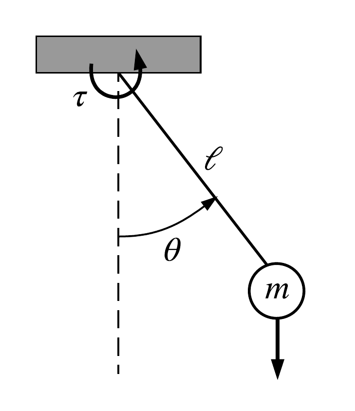
m\ell^2\ddot{\theta}+b\dot{\theta}+mg\ell\sin\theta=0
(péndulo simple con fricción)
Complicando la situación a una 2D
m\ell^2\ddot{\theta}+b\dot{\theta}+mg\ell\sin\theta=0
(péndulo simple con fricción)
¿Estado del sistema?
x_1=\theta, \quad x_2=\dot{\theta}
2do orden pero \(\dot{\mathbf{x}}=\mathbf{f}(\mathbf{x})\) es de 1er orden, ¿Qué podemos hacer?
\begin{aligned} & \dot{x}_1=\dot{\theta}=x_2 \\
& \dot{x}_2=\ddot{\theta}=-\frac{b}{m\ell^2}\dot{\theta}-\frac{g}{\ell}\sin\theta=-\frac{b}{m\ell^2}x_2-\frac{g}{\ell}\sin{x_1} \end{aligned}
\begin{aligned} & \dot{x}_1=\dot{\theta}=x_2 \\
& \dot{x}_2=\ddot{\theta}=-\frac{b}{m\ell^2}\dot{\theta}-\frac{g}{\ell}\sin\theta=-\frac{b}{m\ell^2}x_2-\frac{g}{\ell}\sin{x_1} \end{aligned}
\Rightarrow \begin{bmatrix} \dot{x}_1 \\ \dot{x}_2 \end{bmatrix}=
\begin{bmatrix} x_2 \\ -\frac{g}{\ell}\sin{x_1}-\frac{b}{m\ell^2}x_2 \end{bmatrix}
\dot{\mathbf{x}}
\mathbf{f}\left(\mathbf{x}\right)
\begin{cases} \dot{\mathbf{x}}=\mathbf{f}\left(\mathbf{x}\right) \\ \mathbf{x}(t_0)=\mathbf{x}_0 \end{cases}
\begin{aligned} & \dot{x}_1=\dot{\theta}=x_2 \\
& \dot{x}_2=\ddot{\theta}=-\frac{b}{m\ell^2}\dot{\theta}-\frac{g}{\ell}\sin\theta=-\frac{b}{m\ell^2}x_2-\frac{g}{\ell}\sin{x_1} \end{aligned}
¿Tiene solución este IVP?
NO
\Rightarrow \begin{bmatrix} \dot{x}_1 \\ \dot{x}_2 \end{bmatrix}=
\begin{bmatrix} x_2 \\ -\frac{g}{\ell}\sin{x_1}-\frac{b}{m\ell^2}x_2 \end{bmatrix}
\dot{\mathbf{x}}
\mathbf{f}\left(\mathbf{x}\right)
\begin{cases} \dot{\mathbf{x}}=\mathbf{f}\left(\mathbf{x}\right) \\ \mathbf{x}(t_0)=\mathbf{x}_0 \end{cases}
¿Por qué?
\begin{cases} \dot{\mathbf{x}}=\mathbf{f}\left(\mathbf{x}\right) \\ \mathbf{x}(t_0)=\mathbf{x}_0 \end{cases}
\displaystyle \int_{t_0}^{t} \dot{\mathbf{x}}(\tau) d\tau=
\displaystyle \int_{t_0}^{t} \mathbf{f}\left(\mathbf{x}(\tau)\right) d\tau
¿Por qué?
\begin{cases} \dot{\mathbf{x}}=\mathbf{f}\left(\mathbf{x}\right) \\ \mathbf{x}(t_0)=\mathbf{x}_0 \end{cases}
\displaystyle \int_{t_0}^{t} \dot{\mathbf{x}}(\tau) d\tau=
\displaystyle \int_{t_0}^{t} \mathbf{f}\left(\mathbf{x}(\tau)\right) d\tau
\mathbf{x}(t)=
\mathbf{x}(t_0) + \displaystyle \int_{t_0}^{t} \mathbf{f}\left(\mathbf{x}(\tau)\right) d\tau
???
¿Por qué?
\begin{cases} \dot{\mathbf{x}}=\mathbf{f}\left(\mathbf{x}\right) \\ \mathbf{x}(t_0)=\mathbf{x}_0 \end{cases}
\displaystyle \int_{t_0}^{t} \dot{\mathbf{x}}(\tau) d\tau=
\displaystyle \int_{t_0}^{t} \mathbf{f}\left(\mathbf{x}(\tau)\right) d\tau
\mathbf{x}(t)=
\mathbf{x}(t_0) + \displaystyle \int_{t_0}^{t} \mathbf{f}\left(\mathbf{x}(\tau)\right) d\tau
en general NO tiene solución analítica
¿Qué ocurre en el espacio de estados?
\ x_1
0
1
2
3
-1
-2
x_2
1
-1
¿Qué ocurre en el espacio de estados?
\ x_1
0
1
2
3
-1
-2
x_2
1
-1
\left. \dot{\mathbf{x}} \right\vert_{\mathbf{x}=\begin{bmatrix} 0 \\ 1 \end{bmatrix}}=
\mathbf{f}\left( \begin{bmatrix} 0 \\ 1 \end{bmatrix} \right)=
\begin{bmatrix} 1 \\ -\frac{b}{m\ell^2} \end{bmatrix}
¿Qué ocurre en el espacio de estados?
\ x_1
0
1
2
3
-1
-2
x_2
1
-1
\left. \dot{\mathbf{x}} \right\vert_{\mathbf{x}=\begin{bmatrix} 0 \\ 1 \end{bmatrix}}=
\mathbf{f}\left( \begin{bmatrix} 0 \\ 1 \end{bmatrix} \right)=
\begin{bmatrix} 1 \\ -\frac{b}{m\ell^2} \end{bmatrix}
y puede repetirse (tediosamente) el procedimiento como para el caso 1D
Sin embargo, ¿No puede explotarse que la representación en variables de estado sea amigable a métodos numéricos?
¿Qué ocurre en el espacio de estados?
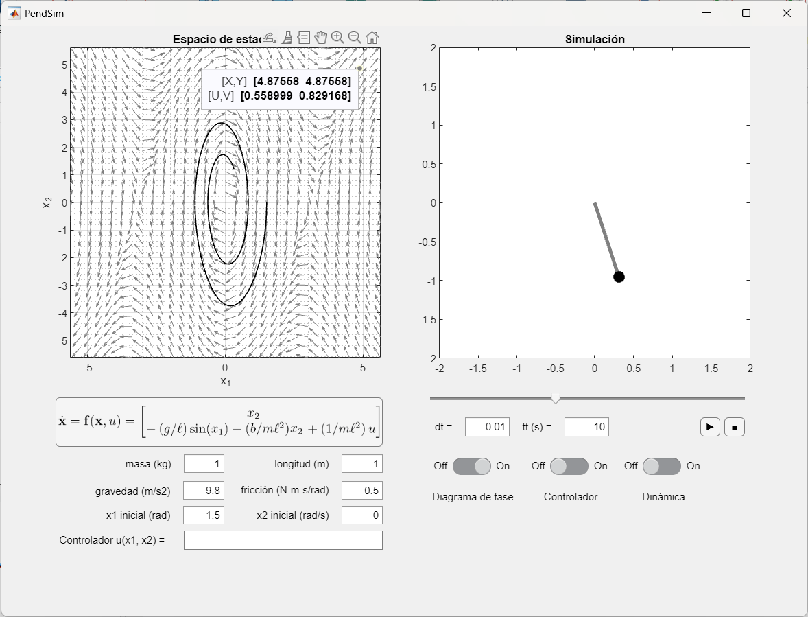
PendSim en MATLAB
(también permite entradas)
Aún mayor complejidad (en 3D)
\begin{aligned} & \dot{x}=\sigma(y-x) \\
& \dot{y}=x(\rho-z)-y \\
& \dot{z}=xy-\beta z \end{aligned}
(sistema de Lorenz)
Aún mayor complejidad (en 3D)
\begin{aligned} & \dot{x}=\sigma(y-x) \\
& \dot{y}=x(\rho-z)-y \\
& \dot{z}=xy-\beta z \end{aligned}
\begin{bmatrix} \dot{x}_1 \\ \dot{x}_2 \\ \dot{x}_3 \end{bmatrix}
=\begin{bmatrix} \sigma(x_2-x_1) \\ x_1(\rho-x_3)-x_2 \\ x_1 x_2-\beta x_3 \end{bmatrix}
(sistema de Lorenz)
\dot{\mathbf{x}}
\mathbf{f}\left(\mathbf{x}\right)
¿Solución? ¿Diagrama de fase?
¿Solución? ¿Diagrama de fase?
Simulación
\mathbf{x}(t)=\mathbf{x}(t_0)+\displaystyle\int_{t_0}^{t}\mathbf{f}\left(\mathbf{x}(\tau)\right) d\tau
0
k\Delta t
(k+1)\Delta t
+
\Delta t
k
k+1
c.t.
d.t.
Simulación
\mathbf{x}(t)=\mathbf{x}(t_0)+\displaystyle\int_{t_0}^{t}\mathbf{f}\left(\mathbf{x}(\tau)\right) d\tau
0
k\Delta t
(k+1)\Delta t
+
\Delta t
k
k+1
c.t.
d.t.
\Rightarrow \mathbf{x}_{k+1}=\mathbf{x}_k+\displaystyle\int_{\Delta t}\mathbf{f}\left(\mathbf{x}(\tau)\right) d\tau
Simulación
\mathbf{x}(t)=\mathbf{x}(t_0)+\displaystyle\int_{t_0}^{t}\mathbf{f}\left(\mathbf{x}(\tau)\right) d\tau
0
k\Delta t
(k+1)\Delta t
+
\Delta t
k
k+1
c.t.
d.t.
\Rightarrow \mathbf{x}_{k+1}=\mathbf{x}_k+\displaystyle\int_{\Delta t}\mathbf{f}\left(\mathbf{x}(\tau)\right) d\tau
\displaystyle\int_{\Delta t}\mathbf{f}\left(\mathbf{x}(\tau)\right) d\tau \approx
\mathbf{f}\left(\mathbf{x}_k\right)\Delta t
\dfrac{\Delta t}{6}(k_1+2k_2+2k_3+k_4)
forward Euler
Runge-Kutta orden 4 (RK4)
\mathbf{x}_{k+1}=\mathbf{x}_k+\mathbf{f}\left(\mathbf{x}_k\right)\Delta t
\mathbf{x}_{k+1}=\mathbf{x}_k+\dfrac{\Delta t}{6}(k_1+2k_2+2k_3+k_4)
forward Euler
k_1=\mathbf{f}\left(\mathbf{x}_k\right)
k_2=\mathbf{f}\left(\mathbf{x}_k+\dfrac{\Delta t}{2}k_1\right)
k_3=\mathbf{f}\left(\mathbf{x}_k+\dfrac{\Delta t}{2}k_2\right)
k_4=\mathbf{f}\left(\mathbf{x}_k+\Delta t k_3\right)
RK4
>> ie3041_clase1_lorenz.mlx
\mathbf{x}_{k+1}=\mathbf{x}_k+\mathbf{f}\left(\mathbf{x}_k\right)\Delta t
\mathbf{x}_{k+1}=\mathbf{x}_k+\dfrac{\Delta t}{6}(k_1+2k_2+2k_3+k_4)
forward Euler
k_1=\mathbf{f}\left(\mathbf{x}_k\right)
k_2=\mathbf{f}\left(\mathbf{x}_k+\dfrac{\Delta t}{2}k_1\right)
k_3=\mathbf{f}\left(\mathbf{x}_k+\dfrac{\Delta t}{2}k_2\right)
k_4=\mathbf{f}\left(\mathbf{x}_k+\Delta t k_3\right)
RK4
en general
\mathbf{x}_{k+1}=\mathbf{F}\left(\mathbf{x}_k\right)
mapa iterado o sistema dinámico (no lineal) discreto en el tiempo
¿Conclusión?
sistemas no lineales \(\Leftrightarrow\) sistemas complicados
¿Solución?
¿Conclusión?
sistemas no lineales \(\Leftrightarrow\) sistemas complicados
¿Solución?
Sistemas LTI
IE3041 - Lecture 1 (2025)
By Miguel Enrique Zea Arenales


