


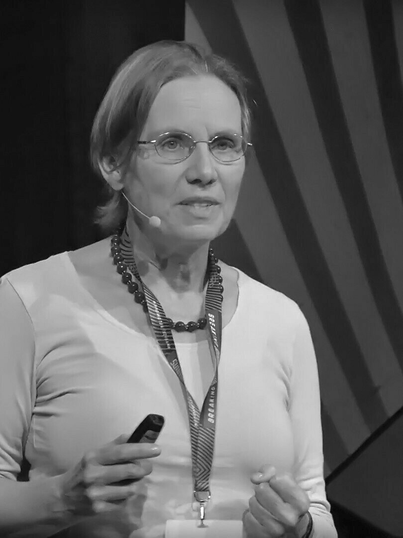


Jeanne Colbois PRO
Physicist @ CNRS. Here you find slides for *some* of my presentations, as well as visual abstracts for recent publications.
Jeanne Colbois | TMC
Jeanne Colbois | TMC
Tensor networks
Jeanne Colbois | TMC
Ising model(s)
Tensor networks
Frustrated magnetism
Jeanne Colbois | TMC
Ising model(s)
Tensor networks
Frustrated magnetism
Jeanne Colbois | TMC
Ising model(s)
Tensor networks
Frustrated magnetism
Jeanne Colbois | TMC
Ising model(s)
Tensor networks
Frustrated magnetism
1
COLBOIS| ISING, ICE AND DOMINOES | 09.2025
1
COLBOIS| ISING, ICE AND DOMINOES | 09.2025
1
COLBOIS| ISING, ICE AND DOMINOES | 09.2025
1
COLBOIS| ISING, ICE AND DOMINOES | 09.2025
1
COLBOIS| ISING, ICE AND DOMINOES | 09.2025
Toy models,
effective hamiltonians
1
COLBOIS| ISING, ICE AND DOMINOES | 09.2025
Toy models,
effective hamiltonians
partition function
2
COLBOIS| ISING, ICE AND DOMINOES | 09.2025
2
Frustration
in artificial spin systems
PhD : Emergent disorder
2017-2022
Frédéric Mila
COLBOIS| ISING, ICE AND DOMINOES | 09.2025
2
Frustration
in artificial spin systems
PhD : Emergent disorder
Tensor networks + Monte Carlo
Tensor networks to demonstrate magnetic disorder at zero temperature
2017-2022
Frédéric Mila
COLBOIS| ISING, ICE AND DOMINOES | 09.2025
2
Frustration
in artificial spin systems
PhD : Emergent disorder
Postdocs : quenched disorder in spin chains
Tensor networks + Monte Carlo
Tensor networks to demonstrate magnetic disorder at zero temperature
2022-2024
2017-2022
Frédéric Mila
COLBOIS| ISING, ICE AND DOMINOES | 09.2025
2
Anderson &
Many-body localization
Frustration
in artificial spin systems
PhD : Emergent disorder
Postdocs : quenched disorder in spin chains
Tensor networks + Monte Carlo
"Shift-invert" exact diagonalization
Tensor networks to demonstrate magnetic disorder at zero temperature
2022-2024
2017-2022
Frédéric Mila
Nicolas Laflorencie
Fabien Alet
Instability of Anderson
localization to weak interactions
vs Many-body localization
COLBOIS| ISING, ICE AND DOMINOES | 09.2025
2
Anderson &
Many-body localization
Frustration
in artificial spin systems
PhD : Emergent disorder
Postdocs : quenched disorder in spin chains
Tensor networks + Monte Carlo
"Shift-invert" exact diagonalization
Localization,
Glassy physics
DMRG
Tensor networks to demonstrate magnetic disorder at zero temperature
Localization transitions from extreme statistics
2022-2024
2017-2022
Frédéric Mila
Nicolas Laflorencie
Fabien Alet
Gabriel Lemarié
Shaffique Adam
Instability of Anderson
localization to weak interactions
vs Many-body localization
COLBOIS| ISING, ICE AND DOMINOES | 09.2025
3
Tensor network investigation of fragmented magnetism
Each spin participates to both phases!
Magnetic order
Spin
liquid
COLBOIS| ISING, ICE AND DOMINOES | 09.2025
3
Tensor network investigation of fragmented magnetism
Each spin participates to both phases!
Magnetic order
Spin
liquid
Benjamin Canals
Matthieu Deschamps
COLBOIS| ISING, ICE AND DOMINOES | 09.2025
3
Tensor network investigation of fragmented magnetism
Each spin participates to both phases!
Magnetic order
Spin
liquid
Benjamin Canals
Matthieu Deschamps
COLBOIS| ISING, ICE AND DOMINOES | 09.2025
Arnaud Ralko
Remy Dangoisse
... and more frustrated systems !
Laurent Del Rey
Philippe David
Valérie Guisset
Johann Coraux
Nicolas Rougemaille
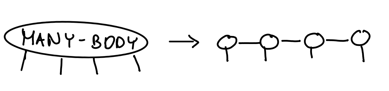
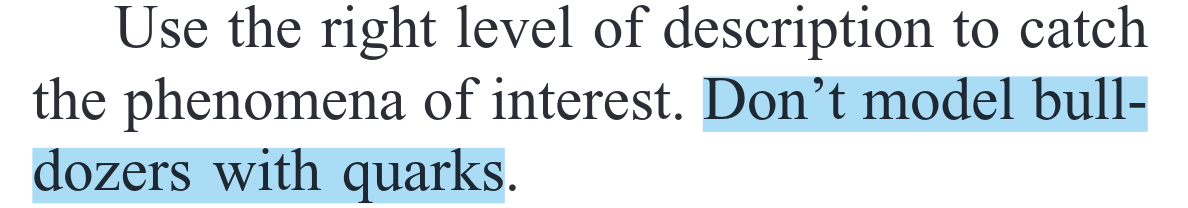
1. Why study Ising models?
2. Tensor networks and the many-body problem
3. Tensor networks should work for Ising models
4. Frustrated models as domino games
5. Some applications & perspectives
4
COLBOIS| ISING, ICE AND DOMINOES | 09.2025
Why it matters
Why we want to solve it
Why it is hard
5
COLBOIS| ISING, ICE AND DOMINOES | 09.2025
\(\sigma_i\) is the orientation of a spin
Lenz (1920), Ising (1925)
5
COLBOIS| ISING, ICE AND DOMINOES | 09.2025
\(\sigma_i\) is the orientation of a spin
Lenz (1920), Ising (1925)
5
COLBOIS| ISING, ICE AND DOMINOES | 09.2025
\(\sigma_i\) is the orientation of a spin
Lenz (1920), Ising (1925)
\(T>T_c\)
\(T= T_c\)
\(T< T_c\)
5
COLBOIS| ISING, ICE AND DOMINOES | 09.2025
\(\sigma_i\) is the orientation of a spin
Lenz (1920), Ising (1925)
Real space
\(T>T_c\)
\(T= T_c\)
\(T< T_c\)
5
COLBOIS| ISING, ICE AND DOMINOES | 09.2025
\(\sigma_i\) is the orientation of a spin
Lenz (1920), Ising (1925)
Paramagnet
~ Gas
Real space
Diffraction
Reciprocal space
\(T>T_c\)
\(T= T_c\)
\(T< T_c\)
\(q_x\)
\(q_y\)
\(\xi = 0\)
5
COLBOIS| ISING, ICE AND DOMINOES | 09.2025
\(\sigma_i\) is the orientation of a spin
Lenz (1920), Ising (1925)
Paramagnet
~ Gas
Real space
Diffraction
Reciprocal space
\(T>T_c\)
\(T= T_c\)
\(T< T_c\)
\(q_x\)
\(q_y\)
\(\xi = 0\)
Scale invariance!
5
COLBOIS| ISING, ICE AND DOMINOES | 09.2025
\(\sigma_i\) is the orientation of a spin
Lenz (1920), Ising (1925)
Paramagnet
~ Gas
Real space
Diffraction
Reciprocal space
\(T>T_c\)
\(T= T_c\)
\(T< T_c\)
\(q_x\)
\(q_y\)
\(\xi = 0\)
Scale invariance!
5
COLBOIS| ISING, ICE AND DOMINOES | 09.2025
\(\sigma_i\) is the orientation of a spin
Lenz (1920), Ising (1925)
Paramagnet
~ Gas
Real space
Diffraction
Reciprocal space
\(T>T_c\)
\(T= T_c\)
\(T< T_c\)
\(q_x\)
\(q_y\)
\(\xi = 0\)
Magnetic order
~ solid
\(q_x\)
\(\xi = \infty\)
\(q_y\)
Scale invariance!
6
COLBOIS| ISING, ICE AND DOMINOES | 09.2025
6
COLBOIS| ISING, ICE AND DOMINOES | 09.2025
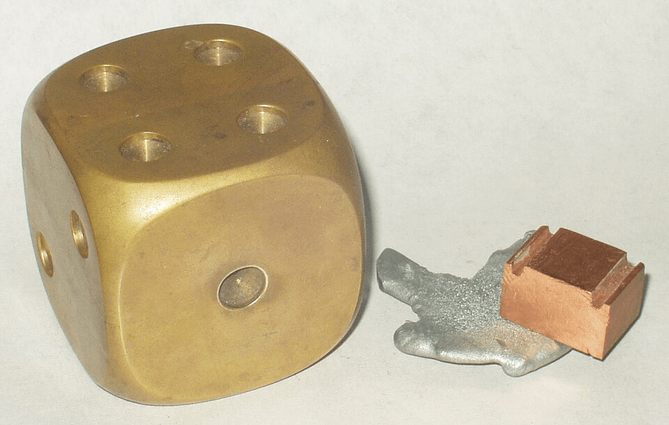
Wikimedia comons
Brass!
\(\sigma_i\) : Cu / Zn
Madsen et al PRB 2016
Same behavior at the transition!
(Ordered to disordered sublattice occupation)
6
COLBOIS| ISING, ICE AND DOMINOES | 09.2025
Hopfield networks
Voter models
\(\sigma_i\) : opinion
\(\sigma_i\) : off / on neuron
Wikimedia comons
\(\sigma_i\) : Cu / Zn
Madsen et al PRB 2016
Same behavior at the transition!
Brass!
(Ordered to disordered sublattice occupation)
(c.f Nobel 2024)
7
COLBOIS| ISING, ICE AND DOMINOES | 09.2025
7
COLBOIS| ISING, ICE AND DOMINOES | 09.2025
Solid : only a few configurations in the ground state.
7
COLBOIS| ISING, ICE AND DOMINOES | 09.2025
Solid : only a few configurations in the ground state.
Giauque and Ashley, (1933)
7
COLBOIS| ISING, ICE AND DOMINOES | 09.2025
Giauque and Ashley, (1933)
Bernal and Fowler, (1933)
Solid : only a few configurations in the ground state.
Lattice of oxygens
COLBOIS| ISING, ICE AND DOMINOES | 09.2025
Giauque and Ashley, (1933)
Bernal and Fowler, (1933)
Solid : only a few configurations in the ground state.
7
Lattice of oxygens
Hydrogens form the molecules...
COLBOIS| ISING, ICE AND DOMINOES | 09.2025
Giauque and Ashley, (1933)
Bernal and Fowler, (1933)
7
Lattice of oxygens
Hydrogens form the molecules...
Solid : only a few configurations in the ground state.
COLBOIS| ISING, ICE AND DOMINOES | 09.2025
Giauque and Ashley, (1933)
Bernal and Fowler, (1933)
... under constraints:
1 hydrogen / bond
7
Solid : only a few configurations in the ground state.
Lattice of oxygens
Hydrogens form the molecules...
COLBOIS| ISING, ICE AND DOMINOES | 09.2025
Giauque and Ashley, (1933)
Bernal and Fowler, (1933)
... under constraints:
1 hydrogen / bond
7
Solid : only a few configurations in the ground state.
Lattice of oxygens
Hydrogens form the molecules...
COLBOIS| ISING, ICE AND DOMINOES | 09.2025
Giauque and Ashley, (1933)
Bernal and Fowler, (1933)
... under constraints:
1 hydrogen / bond
7
Solid : only a few configurations in the ground state.
Lattice of oxygens
Hydrogens form the molecules...
Pauling (1935)
COLBOIS| ISING, ICE AND DOMINOES | 09.2025
Giauque and Ashley, (1933)
Bernal and Fowler, (1933)
... under constraints:
1 hydrogen / bond
7
Solid : only a few configurations in the ground state.
Lattice of oxygens
Hydrogens form the molecules...
All hydrogen configurations
Pauling (1935)
COLBOIS| ISING, ICE AND DOMINOES | 09.2025
Giauque and Ashley, (1933)
Bernal and Fowler, (1933)
... under constraints:
1 hydrogen / bond
7
Solid : only a few configurations in the ground state.
Lattice of oxygens
Hydrogens form the molecules...
All hydrogen configurations
Valid configurations in tetrahedrons
Pauling (1935)
\(\sim 2^{3\cdot 10^{23}}\) configurations in your ice cube
vs \(\sim 2^{265}\) atoms in the universe
8
COLBOIS| ISING, ICE AND DOMINOES | 09.2025
COLBOIS| ISING, ICE AND DOMINOES | 09.2025
Ramirez et al (1999) : Dy2Ti2O7
8
COLBOIS| ISING, ICE AND DOMINOES | 09.2025
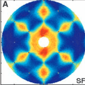
Ramirez et al (1999) : Dy2Ti2O7
\(\xi = \infty\)
Reciprocal space
Fennell et al. (2009) Ho2Ti2O7
8
COLBOIS| ISING, ICE AND DOMINOES | 09.2025
Ramirez et al (1999) : Dy2Ti2O7
\(\xi = \infty\)
Reciprocal space
Fennell et al. (2009) Ho2Ti2O7
8
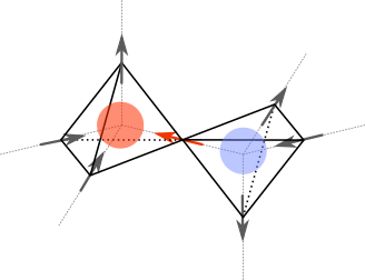
Gauss law \(\nabla \cdot \mathbf{B} = 0\)
COLBOIS| ISING, ICE AND DOMINOES | 09.2025
Ramirez et al (1999) : Dy2Ti2O7
\(\xi = \infty\)
Reciprocal space
Fennell et al. (2009) Ho2Ti2O7
Spin flip : 2 charges
Effective Coulomb interaction
\(|F| \propto q^2/r^2\)
8
Henley (2005, 2010), Castelnovo etal(2008)...
Gauss law \(\nabla \cdot \mathbf{B} = 0\)
Classical / quantum electrodynamics
COLBOIS| ISING, ICE AND DOMINOES | 09.2025
9
M. Zhu et al, PRL (2024), NPJ quantum materials (2025)
COLBOIS| ISING, ICE AND DOMINOES | 09.2025
9
M. Zhu et al, PRL (2024), NPJ quantum materials (2025)
Spin up
Spin down
M. Zhu et al, PRL (2024), NPJ quantum materials (2025)
COLBOIS| ISING, ICE AND DOMINOES | 09.2025
9
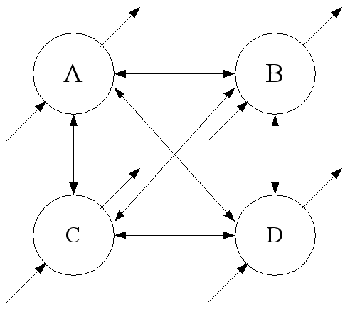
Wannier, Houttapel (1950)
With field: Blöte et al (1993), Qian et al (2004), Nyckees et al (JC) (2023)
M. Zhu et al, PRL (2024), NPJ quantum materials (2025)
Spin up
Spin down
COLBOIS| ISING, ICE AND DOMINOES | 09.2025
9
Wannier, Houttapel (1950)
With field: Blöte et al (1993), Qian et al (2004), Nyckees et al (JC) (2023)
M. Zhu et al, PRL (2024), NPJ quantum materials (2025)
COLBOIS| ISING, ICE AND DOMINOES | 09.2025
9
Wannier, Houttapel (1950)
With field: Blöte et al (1993), Qian et al (2004), Nyckees et al (JC) (2023)
M. Zhu et al, PRL (2024), NPJ quantum materials (2025)
COLBOIS| ISING, ICE AND DOMINOES | 09.2025
9
M. Zhu et al, PRL (2024), NPJ quantum materials (2025)
Wannier, Houttapel (1950)
With field: Blöte et al (1993), Qian et al (2004), Nyckees et al (JC) (2023)
\(\Omega > 2^{N/3}\)
COLBOIS| ISING, ICE AND DOMINOES | 09.2025
10
COLBOIS| ISING, ICE AND DOMINOES | 09.2025
10
COLBOIS| ISING, ICE AND DOMINOES | 09.2025
10
1D Ising
Solved exactly 1925
\(2\)x\(2\)
Ising
1D Ising
Solved exactly 1925
2D Ising
Solved exactly 1944
\(2\)x\(2\)
\(2^{N}\)x\(2^{N}\)
COLBOIS| ISING, ICE AND DOMINOES | 09.2025
10
Ising
Onsager
1D Ising
Solved exactly 1925
2D Ising
Solved exactly 1944
3D Ising
No closed form
2D Ising with a field
No closed form
\(2\)x\(2\)
\(2^{N}\)x\(2^{N}\)
COLBOIS| ISING, ICE AND DOMINOES | 09.2025
10
Ising
Onsager
1D Ising
Solved exactly 1925
2D Ising
Solved exactly 1944
3D Ising
No closed form
2D Ising with a field
No closed form
\(2\)x\(2\)
\(2^{N}\)x\(2^{N}\)
COLBOIS| ISING, ICE AND DOMINOES | 09.2025
10
Ising
Onsager
1D Ising
Solved exactly 1925
2D Ising
Solved exactly 1944
3D Ising
No closed form
2D Ising with a field
No closed form
\(2\)x\(2\)
\(2^{N}\)x\(2^{N}\)
COLBOIS| ISING, ICE AND DOMINOES | 09.2025
10
Ising
Onsager
1D Ising
Solved exactly 1925
2D Ising
Solved exactly 1944
3D Ising
No closed form
2D Ising with a field
No closed form
\(2\)x\(2\)
\(2^{N}\)x\(2^{N}\)
COLBOIS| ISING, ICE AND DOMINOES | 09.2025
10
Ising
Onsager
Spin glasses
Counting the number of ground states:
#P-complete
(#P : asking how-many solutions in an NP problem.)
Barahona (1982)
1D Ising
Solved exactly 1925
2D Ising
Solved exactly 1944
3D Ising
No closed form
2D Ising with a field
No closed form
Spin glasses
\(2\)x\(2\)
\(2^{N}\)x\(2^{N}\)
Counting the number of ground states:
#P-complete
(#P : asking how-many solutions in an NP problem.)
Approximate methods: Monte Carlo, series expansion, field theory at the critical point, RG & conformal bootstrap, and...
COLBOIS| ISING, ICE AND DOMINOES | 09.2025
10
Ising
Onsager
Barahona (1982)
What is a tensor network ?
Why do tensor networks matter?
What are key concepts ?
11
COLBOIS| ISING, ICE AND DOMINOES | 09.2025
11
COLBOIS| ISING, ICE AND DOMINOES | 09.2025
11
COLBOIS| ISING, ICE AND DOMINOES | 09.2025
11
COLBOIS| ISING, ICE AND DOMINOES | 09.2025
11
COLBOIS| ISING, ICE AND DOMINOES | 09.2025
1D quantum many-body
\(S=1\) Heisenberg chain
Frustrated spin ladders
Disordered chains
...
White (1992), ...
11
COLBOIS| ISING, ICE AND DOMINOES | 09.2025
1D quantum many-body
2D and more quantum many-body
\(S=1\) Heisenberg chain
Frustrated spin ladders
Disordered chains
...
Topological order
Two-dimensional t-J model
Magnetization plateaus in Shastry-Sutherland
White (1992), ...
Verstraete et al (2004), Corboz (2014), ....
11
COLBOIS| ISING, ICE AND DOMINOES | 09.2025
1D quantum many-body
2D and more quantum many-body
Quantum computing
\(S=1\) Heisenberg chain
Frustrated spin ladders
Disordered chains
...
Topological order
Two-dimensional t-J model
Magnetization plateaus in Shastry-Sutherland
Classical simulation of quantum circuits
Challenging quantum supremacy claims
....
White (1992), ...
Verstraete et al (2004), Corboz (2014), ....
Vidal (2003), Zhou, Stoudenmire and Waintal (2020), ...
11
COLBOIS| ISING, ICE AND DOMINOES | 09.2025
1D quantum many-body
2D and more quantum many-body
\(S=1\) Heisenberg chain
Frustrated spin ladders
Disordered chains
...
...and many more...
Topological order
Two-dimensional t-J model
Magnetization plateaus in Shastry-Sutherland
Classical simulation of quantum circuits
Challenging quantum supremacy claims
....
White (1992), ...
Verstraete et al (2004), Corboz (2014), ....
Vidal (2003), Zhou, Stoudenmire and Waintal (2020), ...
Chemistry, machine learning, mathematics...
Quantum computing
12
COLBOIS| ISING, ICE AND DOMINOES | 09.2025
Tensor notation: R. Penrose, in Combinatorial Mathematics and its applications, (1971)
Type
Notation
Visualization
Tensor notation: R. Penrose, in Combinatorial Mathematics and its applications, (1971)
Scalar
Vector
Type
Notation
Visualization
Matrix
Rank-3 tensor
"Legs"
12
COLBOIS| ISING, ICE AND DOMINOES | 09.2025
Tensor notation: R. Penrose, in Combinatorial Mathematics and its applications, (1971)
Scalar
Vector
Type
Notation
Visualization
Matrix
Rank-3 tensor
"Legs"
12
COLBOIS| ISING, ICE AND DOMINOES | 09.2025
Tensor notation: R. Penrose, in Combinatorial Mathematics and its applications, (1971)
Scalar
Vector
Type
Notation
Visualization
Matrix
Rank = # indices = # legs =#dimensions
Rank-3 tensor
"Legs"
12
COLBOIS| ISING, ICE AND DOMINOES | 09.2025
Tensor notation: R. Penrose, in Combinatorial Mathematics and its applications, (1971)
Scalar
Vector
Type
Notation
Visualization
Matrix
Rank = # indices = # legs =#dimensions
Rank-3 tensor
"Legs"
12
COLBOIS| ISING, ICE AND DOMINOES | 09.2025
Size of the index = bond dimension = \(\chi\) or \(D\)
Tensor notation: R. Penrose, in Combinatorial Mathematics and its applications, (1971)
Scalar
Vector
Type
Notation
Visualization
Matrix
Rank = # indices = # legs =#dimensions
Rank-3 tensor
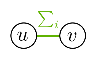
Connecting legs = make the product
"CONTRACTION"
"Legs"
12
COLBOIS| ISING, ICE AND DOMINOES | 09.2025
Size of the index = bond dimension = \(\chi\) or \(D\)
Tensor notation: R. Penrose, in Combinatorial Mathematics and its applications, (1971)
Scalar
Vector
Type
Notation
Visualization
Matrix
Rank = # indices = # legs =#dimensions
Rank-3 tensor
Scalar product
Connecting legs = make the product
"CONTRACTION"
"Legs"
12
COLBOIS| ISING, ICE AND DOMINOES | 09.2025
Size of the index = bond dimension = \(\chi\) or \(D\)
Tensor notation: R. Penrose, in Combinatorial Mathematics and its applications, (1971)
Scalar
Vector
Type
Notation
Visualization
Matrix
Rank = # indices = # legs =#dimensions
Rank-3 tensor
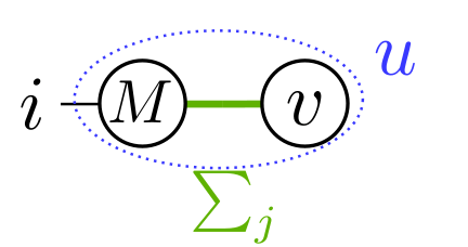
Scalar product
Matrix-vector product
Connecting legs = make the product
"CONTRACTION"
"Legs"
12
COLBOIS| ISING, ICE AND DOMINOES | 09.2025
Size of the index = bond dimension = \(\chi\) or \(D\)
Tensor notation: R. Penrose, in Combinatorial Mathematics and its applications, (1971)
Scalar
Vector
Type
Notation
Visualization
Matrix
Rank = # indices = # legs =#dimensions
Rank-3 tensor
Scalar product
Matrix-vector product
Connecting legs = make the product
"CONTRACTION"
"Legs"
Only 2 legs can meet!
12
COLBOIS| ISING, ICE AND DOMINOES | 09.2025
Size of the index = bond dimension = \(\chi\) or \(D\)
You can group indices:
\(\chi \times\chi \times \chi \times \chi\)
tensor
\(\chi^2 \times\chi^2\)
matrix
13
COLBOIS| ISING, ICE AND DOMINOES | 09.2025
A complicated tensor network product giving a matrix
13
COLBOIS| ISING, ICE AND DOMINOES | 09.2025
A complicated tensor network product giving a matrix
Goldenfeld & Kadanoff, Science, 284 (1999)
13
COLBOIS| ISING, ICE AND DOMINOES | 09.2025
A complicated tensor network product giving a matrix
Goldenfeld & Kadanoff, Science, 284 (1999)
Wikipedia, CC BY license
14
COLBOIS| ISING, ICE AND DOMINOES | 09.2025
Julia Yeomans
\(M\)
\(U\)
\(S\)
\(V\)
\(=\)
Wikipedia, CC BY license
14
COLBOIS| ISING, ICE AND DOMINOES | 09.2025
\(M\)
\(U\)
\(S\)
\(V\)
\(=\)
Wikipedia, CC BY license
14
COLBOIS| ISING, ICE AND DOMINOES | 09.2025
\(M\)
\(U\)
\(S\)
\(V\)
\(=\)
Wikipedia, CC BY license
14
COLBOIS| ISING, ICE AND DOMINOES | 09.2025
\(M\)
\(U\)
\(S\)
\(V\)
\(=\)
Wikipedia, CC BY license
COLBOIS| ISING, ICE AND DOMINOES | 09.2025
14
\(M\)
\(U\)
\(S\)
\(V\)
\(=\)
Wikipedia, CC BY license
COLBOIS| ISING, ICE AND DOMINOES | 09.2025
14
\(M\)
\(U\)
\(S\)
\(V\)
\(=\)
Wikipedia, CC BY license
COLBOIS| ISING, ICE AND DOMINOES | 09.2025
\(\chi = 4\)
14
\(M\)
\(U\)
\(S\)
\(V\)
\(=\)
Wikipedia, CC BY license
COLBOIS| ISING, ICE AND DOMINOES | 09.2025
\(\chi = 4\)
\(\chi = 20\)
14
\(M\)
\(U\)
\(S\)
\(V\)
\(=\)
Wikipedia, CC BY license
COLBOIS| ISING, ICE AND DOMINOES | 09.2025
\(\chi = 4\)
\(\chi = 20\)
\(\chi = 100\)
14
\(M\)
\(U\)
\(S\)
\(V\)
\(=\)
Wikipedia, CC BY license
COLBOIS| ISING, ICE AND DOMINOES | 09.2025
\(\chi = 4\)
\(\chi = 20\)
\(\chi = 100\)
14
\(M\)
\(U\)
\(S\)
\(V\)
\(=\)
Wikipedia, CC BY license
COLBOIS| ISING, ICE AND DOMINOES | 09.2025
\(\chi = 4\)
\(\chi = 20\)
\(\chi = 100\)
14
COLBOIS| ISING, ICE AND DOMINOES | 09.2025
15
Many-body wavefunction
High number of parameters
COLBOIS| ISING, ICE AND DOMINOES | 09.2025
Many-body wavefunction =huge tensor:
High number of parameters
15
COLBOIS| ISING, ICE AND DOMINOES | 09.2025
Many-body wavefunction =huge tensor:
We want to compress it:
High number of parameters
Much smaller number
15
COLBOIS| ISING, ICE AND DOMINOES | 09.2025
Many-body wavefunction =huge tensor:
We want to compress it:
High number of parameters
Much smaller number
15
COLBOIS| ISING, ICE AND DOMINOES | 09.2025
Many-body wavefunction =huge tensor:
We want to compress it:
High number of parameters
Much smaller number
ENTANGLEMENT (area law)
15
COLBOIS| ISING, ICE AND DOMINOES | 09.2025
Many-body wavefunction =huge tensor:
We want to compress it:
ENTANGLEMENT (area law)
High number of parameters
Much smaller number
Many-body Hilbert space
15
COLBOIS| ISING, ICE AND DOMINOES | 09.2025
Many-body wavefunction =huge tensor:
We want to compress it:
ENTANGLEMENT (area law)
High number of parameters
Much smaller number
Many-body Hilbert space
15
COLBOIS| ISING, ICE AND DOMINOES | 09.2025
Many-body wavefunction =huge tensor:
We want to compress it:
Many-body Hilbert space
ENTANGLEMENT (area law)
High number of parameters
Much smaller number
15
COLBOIS| ISING, ICE AND DOMINOES | 09.2025
Many-body wavefunction =huge tensor:
We want to compress it:
Many-body Hilbert space
Ground states of gapped, local Hamiltonians
ENTANGLEMENT (area law)
High number of parameters
Much smaller number
15
COLBOIS| ISING, ICE AND DOMINOES | 09.2025
Many-body wavefunction =huge tensor:
We want to compress it:
Many-body Hilbert space
Ground states of gapped, local Hamiltonians
ENTANGLEMENT (area law)
High number of parameters
Much smaller number
15
COLBOIS| ISING, ICE AND DOMINOES | 09.2025
Many-body wavefunction =huge tensor:
We want to compress it:
Many-body Hilbert space
Ground states of gapped, local Hamiltonians
ENTANGLEMENT (area law)
High number of parameters
Much smaller number
15
1. The 1D Ising model partition function is a TN
2. The solution of the 2D Ising model is TN-related
3. Successes / failures
16
COLBOIS| ISING, ICE AND DOMINOES | 09.2025
COLBOIS| ISING, ICE AND DOMINOES | 09.2025
16
COLBOIS| ISING, ICE AND DOMINOES | 09.2025
16
COLBOIS| ISING, ICE AND DOMINOES | 09.2025
The partition function is just the exponentiation of a 2x2 matrix!
1. Diagonalize
16
COLBOIS| ISING, ICE AND DOMINOES | 09.2025
The partition function is just the exponentiation of a 2x2 matrix!
1. Diagonalize
2. Compute
16
COLBOIS| ISING, ICE AND DOMINOES | 09.2025
Generalized kronecker \(\delta\) tensor
17
R. J. Baxter, J. Math. Phys. 9, 1968
R. Orús, G. Vidal, PRB 78, 2008
T. Nishino, K. Okunishi, J. Phys. Soc. Jpn 65, 1996
COLBOIS| ISING, ICE AND DOMINOES | 09.2025
Ferromagnet / antiferromagnet: Onsager
In a field : no closed form solution
\(L\)
\(M\)
\(\mathcal{T}\) : \(2^{L} \times 2^{L}\)
\(\mathcal{Z} = \mathcal{T}^{M}\)
(But the amount of information stored: \(2\times 2\times 2\times 2\))
R. J. Baxter, J. Math. Phys. 9, 1968; Orús, Vidal, PRB 78, 2008;
V. Zauner-Stauber et. al. PRB 97,2018; M. Fishman et. al PRB 98, 2018
17
COLBOIS| ISING, ICE AND DOMINOES | 09.2025
\(\mathcal{T}\) : \(2^{L} \times 2^{L}\)
\(\mathcal{Z} = \mathcal{T}^{M}\)
Size : \(2\times 2\times 2\)
R. J. Baxter, J. Math. Phys. 9, 1968; Orús, Vidal, PRB 78, 2008;
V. Zauner-Stauber et. al. PRB 97,2018; M. Fishman et. al PRB 98, 2018
18
COLBOIS| ISING, ICE AND DOMINOES | 09.2025
\(\mathcal{T}\) : \(2^{L} \times 2^{L}\)
\(\mathcal{Z} = \mathcal{T}^{M}\)
Size : \(4\times 2\times 4\)
R. J. Baxter, J. Math. Phys. 9, 1968; Orús, Vidal, PRB 78, 2008;
V. Zauner-Stauber et. al. PRB 97,2018; M. Fishman et. al PRB 98, 2018
18
COLBOIS| ISING, ICE AND DOMINOES | 09.2025
\(\mathcal{T}\) : \(2^{L} \times 2^{L}\)
\(\mathcal{Z} = \mathcal{T}^{M}\)
Size : \(8\times 2\times 8\)
R. J. Baxter, J. Math. Phys. 9, 1968; Orús, Vidal, PRB 78, 2008;
V. Zauner-Stauber et. al. PRB 97,2018; M. Fishman et. al PRB 98, 2018
18
COLBOIS| ISING, ICE AND DOMINOES | 09.2025
\(\mathcal{T}\) : \(2^{L} \times 2^{L}\)
\(\mathcal{Z} = \mathcal{T}^{M}\)
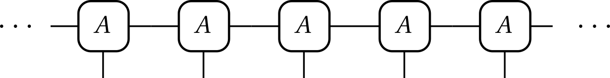
Size : \(2^{r}\times 2\times 2^{r}\)
\(A\)
R. J. Baxter, J. Math. Phys. 9, 1968; Orús, Vidal, PRB 78, 2008;
V. Zauner-Stauber et. al. PRB 97,2018; M. Fishman et. al PRB 98, 2018
18
COLBOIS| ISING, ICE AND DOMINOES | 09.2025
\(\mathcal{T}\) : \(2^{L} \times 2^{L}\)
\(\mathcal{Z} = \mathcal{T}^{M}\)
Size : \(2^{r}\times 2\times 2^{r}\)
\(A\)
Question : can we approximate \(A\) by a \(\chi\times 2\times \chi\) tensor ?
Answer: yes, if the area-law is respected!
18
R. J. Baxter, J. Math. Phys. 9, 1968; Orús, Vidal, PRB 78, 2008;
V. Zauner-Stauber et. al. PRB 97,2018; M. Fishman et. al PRB 98, 2018
COLBOIS| ISING, ICE AND DOMINOES | 09.2025
\(\mathcal{T}\) : \(2^{L} \times 2^{L}\)
\(\mathcal{Z} = \mathcal{T}^{M}\)
Size : \( \chi\times 2\times \chi\)
\(A\)
Question : can we approximate \(A\) by a \(\chi\times 2\times \chi\) tensor ?
Answer: yes, if the area-law is respected!
18
R. J. Baxter, J. Math. Phys. 9, 1968; Orús, Vidal, PRB 78, 2008;
V. Zauner-Stauber et. al. PRB 97,2018; M. Fishman et. al PRB 98, 2018
COLBOIS| ISING, ICE AND DOMINOES | 09.2025
\(\mathcal{Z} = \)
\(A\)
18
R. J. Baxter, J. Math. Phys. 9, 1968; Orús, Vidal, PRB 78, 2008;
V. Zauner-Stauber et. al. PRB 97,2018; M. Fishman et. al PRB 98, 2018
COLBOIS| ISING, ICE AND DOMINOES | 09.2025
\(\mathcal{Z} = \)
19
R. J. Baxter, J. Math. Phys. 9, 1968; Orús, Vidal, PRB 78, 2008;
V. Zauner-Stauber et. al. PRB 97,2018; M. Fishman et. al PRB 98, 2018
COLBOIS| ISING, ICE AND DOMINOES | 09.2025
\(\mathcal{Z} = \)
R. J. Baxter, J. Math. Phys. 9, 1968; Orús, Vidal, PRB 78, 2008;
V. Zauner-Stauber et. al. PRB 97,2018; M. Fishman et. al PRB 98, 2018
19
COLBOIS| ISING, ICE AND DOMINOES | 09.2025
\(\mathcal{Z} = \)
R. J. Baxter, J. Math. Phys. 9, 1968; Orús, Vidal, PRB 78, 2008;
V. Zauner-Stauber et. al. PRB 97,2018; M. Fishman et. al PRB 98, 2018
19
COLBOIS| ISING, ICE AND DOMINOES | 09.2025
\(\mathcal{Z} = \)
\(\overline{m} = \)
Local observable
\(\mathcal{Z}\)
R. J. Baxter, J. Math. Phys. 9, 1968; Orús, Vidal, PRB 78, 2008;
V. Zauner-Stauber et. al. PRB 97,2018; M. Fishman et. al PRB 98, 2018
19
COLBOIS| ISING, ICE AND DOMINOES | 09.2025
2D square lattice Ising model
... and many more, e.g. Huse-Fisher universality class
20
Orús, Vidal, PRB 78, 2008
Nyckees, JC, Mila (2021)
COLBOIS| ISING, ICE AND DOMINOES | 09.2025
2D square lattice Ising model
20
Orús, Vidal, PRB 78, 2008
Vanhecke, JC et al (2021)
... and many more, e.g. Huse-Fisher universality class
Nyckees, JC, Mila (2021)
COLBOIS| ISING, ICE AND DOMINOES | 09.2025
2D square lattice Ising model
20
Orús, Vidal, PRB 78, 2008
Vanhecke, JC et al (2021)
... and many more, e.g. Huse-Fisher universality class
Nyckees, JC, Mila (2021)
COLBOIS| ISING, ICE AND DOMINOES | 09.2025
2D square lattice Ising model
20
Orús, Vidal, PRB 78, 2008
Vanhecke, JC et al (2021)
... and many more, e.g. Huse-Fisher universality class
Nyckees, JC, Mila (2021)
COLBOIS| ISING, ICE AND DOMINOES | 09.2025
2D square lattice Ising model
20
Orús, Vidal, PRB 78, 2008
Vanhecke, JC et al (2021)
... and many more, e.g. Huse-Fisher universality class
Nyckees, JC, Mila (2021)
21
COLBOIS| ISING, ICE AND DOMINOES | 09.2025
COLBOIS| ISING, ICE AND DOMINOES | 09.2025
21
COLBOIS| ISING, ICE AND DOMINOES | 09.2025
21
COLBOIS| ISING, ICE AND DOMINOES | 09.2025
21
COLBOIS| ISING, ICE AND DOMINOES | 09.2025
21
COLBOIS| ISING, ICE AND DOMINOES | 09.2025
21
COLBOIS| ISING, ICE AND DOMINOES | 09.2025
21
COLBOIS| ISING, ICE AND DOMINOES | 09.2025
21
COLBOIS| ISING, ICE AND DOMINOES | 09.2025
21
COLBOIS| ISING, ICE AND DOMINOES | 09.2025
21
COLBOIS| ISING, ICE AND DOMINOES | 09.2025
\(\Omega \approx 1,3385^ N\)
21
Kasteleyn || Temperley & Fisher (1961), R. J. Baxter, (1968)
COLBOIS| ISING, ICE AND DOMINOES | 09.2025
22
\(\Omega \approx 1,3385^ N\)
Kasteleyn || Temperley & Fisher (1961), R. J. Baxter, (1968)
COLBOIS| ISING, ICE AND DOMINOES | 09.2025
\(\Omega \approx 1,3385^ N\)
\(2 \times 2 \times 2 \times 2\)
22
Kasteleyn || Temperley & Fisher (1961), R. J. Baxter, (1968)
COLBOIS| ISING, ICE AND DOMINOES | 09.2025
\(\Omega \approx 1,3385^ N\)
\(2 \times 2 \times 2 \times 2\)
22
Kasteleyn || Temperley & Fisher (1961), R. J. Baxter, (1968)
COLBOIS| ISING, ICE AND DOMINOES | 09.2025
\(\Omega \approx 1,3385^ N\)
\(2 \times 2 \times 2 \times 2\)
22
Kasteleyn || Temperley & Fisher (1961), R. J. Baxter, (1968)
COLBOIS| ISING, ICE AND DOMINOES | 09.2025
\(\Omega \approx 1,3385^ N\)
\(2 \times 2 \times 2 \times 2\)
22
Kasteleyn || Temperley & Fisher (1961), R. J. Baxter, (1968)
COLBOIS| ISING, ICE AND DOMINOES | 09.2025
\(\Omega \approx 1,3385^ N\)
\(2 \times 2 \times 2 \times 2\)
Kasteleyn || Temperley & Fisher (1961), R. J. Baxter, (1968)
22
COLBOIS| ISING, ICE AND DOMINOES | 09.2025
\(\Omega \approx 1,3385^ N\)
\(2 \times 2 \times 2 \times 2\)
Baxter 1968 : First "tensor network" equations to solve this problem.
Kasteleyn || Temperley & Fisher (1961), R. J. Baxter, (1968)
22
23
COLBOIS| ISING, ICE AND DOMINOES | 09.2025
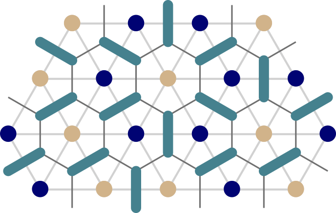
Ground state:
Vanhecke, JC et al (2021)
Kasteleyn, (1961), Fisher (1966)
23
COLBOIS| ISING, ICE AND DOMINOES | 09.2025
Ground state:
Vanhecke, JC et al (2021)
Kasteleyn, (1961), Fisher (1966)
23
COLBOIS| ISING, ICE AND DOMINOES | 09.2025
Ground state:
Vanhecke, JC et al (2021)
Kasteleyn, (1961), Fisher (1966)
Dimer coverings!
23
COLBOIS| ISING, ICE AND DOMINOES | 09.2025
Ground state:
Vanhecke, JC et al (2021)
\(2 \times 2 \times 2\)
\(=0\)
Kasteleyn, (1961), Fisher (1966)
Dimer coverings!
COLBOIS| ISING, ICE AND DOMINOES | 09.2025
Ground state:
Vanhecke, JC et al (2021)
\(2 \times 2 \times 2\)
\(=0\)
Kasteleyn, (1961), Fisher (1966)
23
Dimer coverings!
COLBOIS| ISING, ICE AND DOMINOES | 09.2025
Ground state:
Vanhecke, JC et al (2021)
\(2 \times 2 \times 2\)
\(=0\)
Kasteleyn, (1961), Fisher (1966)
23
Dimer coverings!
COLBOIS| ISING, ICE AND DOMINOES | 09.2025
\(2 \times 2 \times 2\)
Vanhecke, JC et al (2021)
24
COLBOIS| ISING, ICE AND DOMINOES | 09.2025
\(2 \times 2 \times 2\)
Vanhecke, JC et al (2021)
24
COLBOIS| ISING, ICE AND DOMINOES | 09.2025
\(2 \times 2 \times 2\)
Vanhecke, JC et al (2021)
\(=e^{-\beta J}\)
Same structure and size
Different entries
24
COLBOIS| ISING, ICE AND DOMINOES | 09.2025
\(2 \times 2 \times 2\)
Vanhecke, JC et al (2021)
\(=e^{-\beta J}\)
Same structure and size
Different entries
24
COLBOIS| ISING, ICE AND DOMINOES | 09.2025
I. A. Chioar, N. Rougemaille, B. Canals, PRB 93, (2016)
J. Hamp, C. Castelnovo, R. Moessner, PRB 98, (2018)
L. Cugliandolo, L. Foini, M. Tarzia, PRB 101 (2020)
Z. Luo et al. Science 363, (2019)
JC et al., PRB 104 (2021)
25
25
COLBOIS| ISING, ICE AND DOMINOES | 09.2025
I. A. Chioar, N. Rougemaille, B. Canals, PRB 93, (2016)
J. Hamp, C. Castelnovo, R. Moessner, PRB 98, (2018)
L. Cugliandolo, L. Foini, M. Tarzia, PRB 101 (2020)
Z. Luo et al. Science 363, (2019)
JC et al., PRB 104 (2021)
COLBOIS| ISING, ICE AND DOMINOES | 09.2025
I. A. Chioar, N. Rougemaille, B. Canals, PRB 93, (2016)
J. Hamp, C. Castelnovo, R. Moessner, PRB 98, (2018)
L. Cugliandolo, L. Foini, M. Tarzia, PRB 101 (2020)
Z. Luo et al. Science 363, (2019)
JC et al., PRB 104 (2021)
25
COLBOIS| ISING, ICE AND DOMINOES | 09.2025
I. A. Chioar, N. Rougemaille, B. Canals, PRB 93, (2016)
J. Hamp, C. Castelnovo, R. Moessner, PRB 98, (2018)
L. Cugliandolo, L. Foini, M. Tarzia, PRB 101 (2020)
Z. Luo et al. Science 363, (2019)
JC et al., PRB 104 (2021)
25
COLBOIS| ISING, ICE AND DOMINOES | 09.2025
I. A. Chioar, N. Rougemaille, B. Canals, PRB 93, (2016)
J. Hamp, C. Castelnovo, R. Moessner, PRB 98, (2018)
L. Cugliandolo, L. Foini, M. Tarzia, PRB 101 (2020)
Z. Luo et al. Science 363, (2019)
JC et al., PRB 104 (2021)
25
26
COLBOIS| ISING, ICE AND DOMINOES | 09.2025
C. K. Majumdar and D. K. Ghosh, J. Math. Phys. 10, (1969); M. Kaburagi, J. Kanamori, Prog. Theor. Phys. 54 , (1975);
B. Sriram Shastry and B. Sutherland, Physica 108 B+C, (1981); W. Huang, D. A. Kitchaev, et. al. , Phys. Rev. B 94, (2016);
B. Vanhecke, JC, L. Vanderstraeten, F. Verstraete, F. Mila, PRR 3, (2021)
26
COLBOIS| ISING, ICE AND DOMINOES | 09.2025
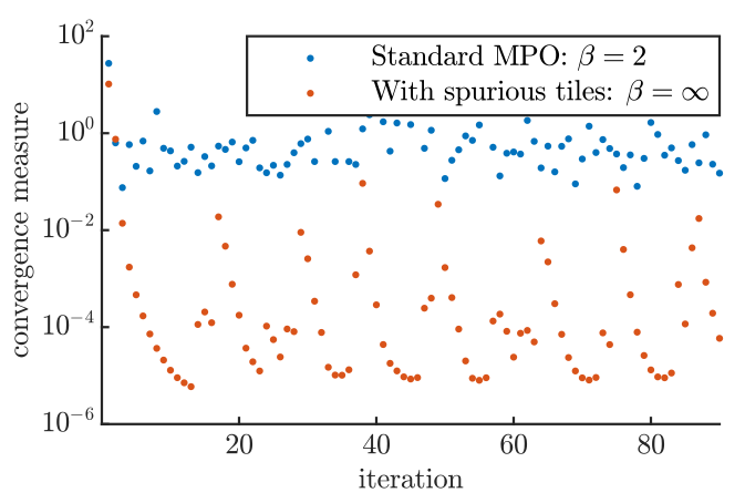
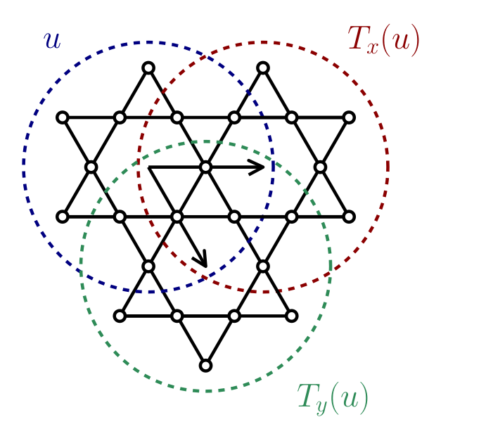
Split the Hamiltonian differently: ground states are tilings of local g.s. configurations!
C. K. Majumdar and D. K. Ghosh, J. Math. Phys. 10, (1969); M. Kaburagi, J. Kanamori, Prog. Theor. Phys. 54 , (1975);
B. Sriram Shastry and B. Sutherland, Physica 108 B+C, (1981); W. Huang, D. A. Kitchaev, et. al. , Phys. Rev. B 94, (2016);
B. Vanhecke, JC, L. Vanderstraeten, F. Verstraete, F. Mila, PRR 3, (2021)
26
COLBOIS| ISING, ICE AND DOMINOES | 09.2025
Split the Hamiltonian differently: ground states are tilings of local g.s. configurations!
C. K. Majumdar and D. K. Ghosh, J. Math. Phys. 10, (1969); M. Kaburagi, J. Kanamori, Prog. Theor. Phys. 54 , (1975);
B. Sriram Shastry and B. Sutherland, Physica 108 B+C, (1981); W. Huang, D. A. Kitchaev, et. al. , Phys. Rev. B 94, (2016);
B. Vanhecke, JC, L. Vanderstraeten, F. Verstraete, F. Mila, PRR 3, (2021)
LINEAR PROGRAM:
26
COLBOIS| ISING, ICE AND DOMINOES | 09.2025
Split the Hamiltonian differently: ground states are tilings of local g.s. configurations!
LINEAR PROGRAM:
C. K. Majumdar and D. K. Ghosh, J. Math. Phys. 10, (1969); M. Kaburagi, J. Kanamori, Prog. Theor. Phys. 54 , (1975);
B. Sriram Shastry and B. Sutherland, Physica 108 B+C, (1981); W. Huang, D. A. Kitchaev, et. al. , Phys. Rev. B 94, (2016);
B. Vanhecke, JC, L. Vanderstraeten, F. Verstraete, F. Mila, PRR 3, (2021)
1. Split the lattice into clusters that overlap
2. Find the optimal energy lower-bound
3. Contract / extend to finite T
COLBOIS| ISING, ICE AND DOMINOES | 09.2025
27
COLBOIS| ISING, ICE AND DOMINOES | 09.2025
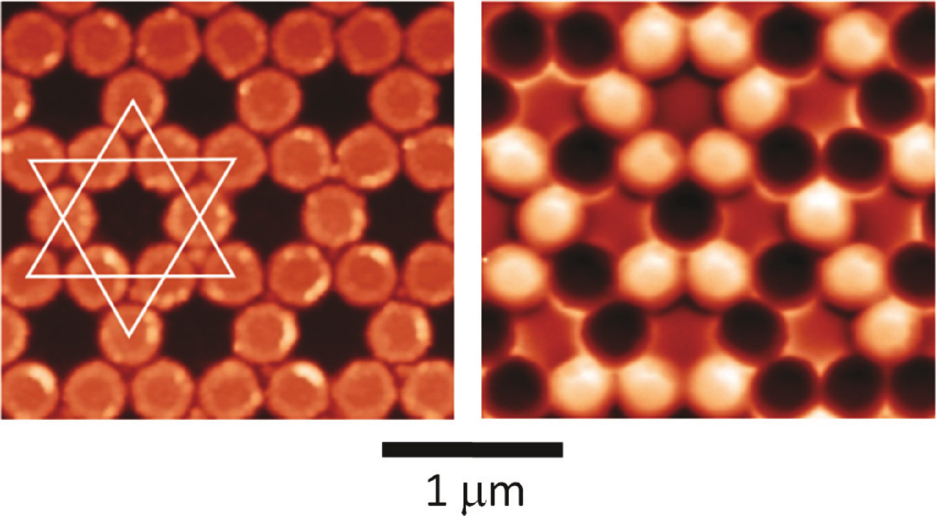
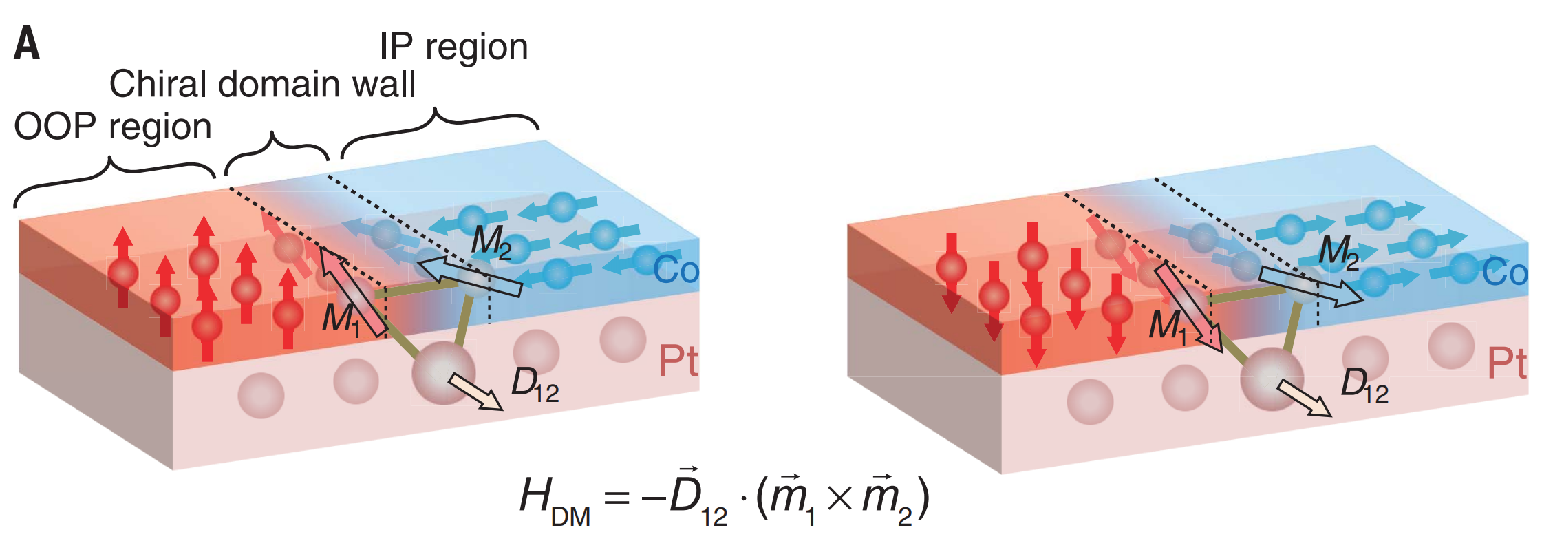
I. A. Chioar, N. Rougemaille, B. Canals, PRB 93, (2016)
J. Hamp, C. Castelnovo, R. Moessner, PRB 98, (2018)
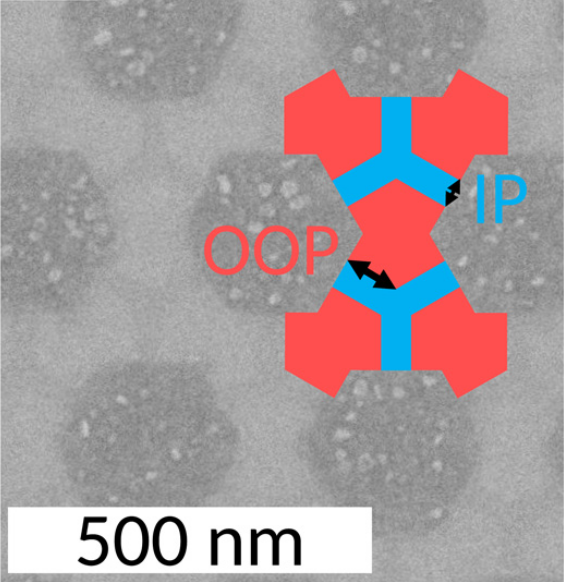
1. Three unexpected spin liquid phases
27
COLBOIS| ISING, ICE AND DOMINOES | 09.2025
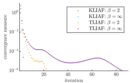
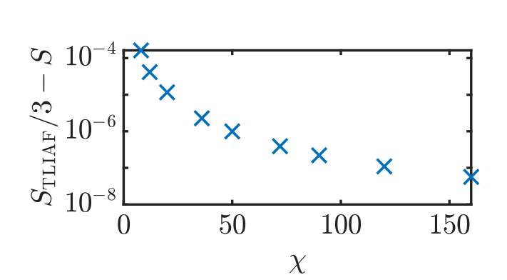
JC, B. Vanhecke et. al., PRB 106 (2022)
1. Three unexpected spin liquid phases
27
COLBOIS| ISING, ICE AND DOMINOES | 09.2025
1. Three unexpected spin liquid phases
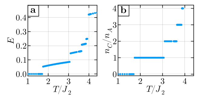
2. Cascade of "topological" phase transitions
JC, B. Vanhecke et. al., PRB 106 (2022)
A. Rufino, S. Nyckees, JC, F. Mila, arXiv:2505.05889 (2025)
27
COLBOIS| ISING, ICE AND DOMINOES | 09.2025
2. Cascade of "topological" phase transitions
Classical XY models for kagome superconductors, Understanding topological order, Studying quantum frustrated magnets, ...
JC, B. Vanhecke et. al., PRB 106 (2022)
A. Rufino, S. Nyckees, JC, F. Mila, arXiv:2505.05889 (2025)
1. Three unexpected spin liquid phases
27
COLBOIS| ISING, ICE AND DOMINOES | 09.2025
28
Tensor network methods
"Classical" and quantum frustrated magnetism
COLBOIS| ISING, ICE AND DOMINOES | 09.2025
28
Tensor network methods
"Classical" and quantum frustrated magnetism
Consequences for studying 2D quantum many-body problems ?
Dealing with non-local constraints ?
Combining with Monte Carlo methods?
Wei Tang et al (2024, 2025)
Châtelain & Gendiar (2020)
Frias-Perez et al (2023)
COLBOIS| ISING, ICE AND DOMINOES | 09.2025
28
Tensor network methods
"Classical" and quantum frustrated magnetism
Consequences for studying 2D quantum many-body problems ?
Dealing with non-local constraints ?
Range of frustration: hard versus "weak" frustration ?
Combining with Monte Carlo methods?
Generalized RK wavefunctions (variational ?) and topology
Wei Tang et al (2024, 2025)
Châtelain & Gendiar (2020)
Frias-Perez et al (2023)
Giudice et al (2022)
Ronceray & Le Floch (2020)
Interpretation of entanglement ?
Carignano et al (2024)
COLBOIS| ISING, ICE AND DOMINOES | 09.2025
29
COLBOIS| ISING, ICE AND DOMINOES | 09.2025
29
Nature can produce complex structures even in simple situations,
COLBOIS| ISING, ICE AND DOMINOES | 09.2025
29
Nature can produce complex structures even in simple situations,
COLBOIS| ISING, ICE AND DOMINOES | 09.2025
Nature can produce complex structures even in simple situations,
and can obey simple laws even in complex situations.
29
COLBOIS| ISING, ICE AND DOMINOES | 09.2025
Tensor networks:
a way to capture those complex structures
Boiling down to simple laws?
29
Nature can produce complex structures even in simple situations,
and can obey simple laws even in complex situations.
By Jeanne Colbois
Seminar at Institut Néel


