The Marginal Rate of Substitution and the Implicit Function Theorem
Christopher Makler
Stanford University Department of Economics
Econ 50: Lecture 3

Special Guest: Monday
Stephen Redding
visiting Stanford from Princeton University
- Research interests include international trade, economic geography, and productivity growth.
- Harold T. Shapiro '64 Professor in Economics in the Economics Department and School of Public and International Affairs at Princeton University;
- Director of the International Trade and Investment (ITI) Program of the National Bureau of Economic Research (NBER);
- Co-Director of the Griswold Center for Economic and Policy Studies (GCEPS) at Princeton University.
QUIZ FOR MONDAY IS DUE SUNDAY NIGHT AT 8PM THIS WEEK ONLY!
previously in Econ 50...
Choices in general
Choices of commodity bundles
Choosing bundles of two goods
Good 1 \((x_1)\)
Good 2 \((x_2)\)
Given any bundle \(A\),
the choice space may be divided
into three regions:
preferred to A
dispreferred to A
indifferent to A
A
The indifference curve through A connects all the bundles indifferent to A.
Indifference curve
through A
Good 1 - Good 2 Space
Good 1 - Good 2 Space
x_1
x_2
Two "Goods" (e.g. apples and bananas)
A bundle is some quantity of each good
\text{Bundle }X = (x_1,x_2)
x_1 = \text{quantity of good 1 in bundle }X
x_2 = \text{quantity of good 2 in bundle }X
Can plot this in a graph with \(x_1\) on the horizontal axis and \(x_2\) on the vertical axis
A = (4,16)
B = (8,8)
A
B
4
8
12
16
20
4
8
12
16
20
Good 1 - Good 2 Space
x_1
x_2
What tradeoff is represented by moving
from bundle A to bundle B?
\text{Give up }\Delta x_2 =
A
B
4
8
12
16
20
4
8
12
16
20
\text{Gain }\Delta x_1 =
\text{Rate of exchange }=
ANY SLOPE IN GOOD 1 - GOOD 2 SPACE
IS MEASURED IN
UNITS OF GOOD 2 PER UNIT OF GOOD 1
ANY SLOPE IN GOOD 1 - GOOD 2 SPACE
IS MEASURED IN
UNITS OF GOOD 2 PER UNIT OF GOOD 1
TW: HORRIBLE STROBE EFFECT!
8 \text{ units of good 2}
4 \text{ units of good 1}
2
\displaystyle{\frac{\text{units of good 2}}{\text{units of good 1}}}
\Delta x_2
\Delta x_1
Marginal Rate of Substitution
X = (10,24)
🍏🍏
🍏🍏
🍏🍏
🍏🍏
🍏🍏
🍌🍌🍌🍌
🍌🍌🍌🍌
🍌🍌🍌🍌
🍌🍌🍌🍌
🍌🍌🍌🍌
🍌🍌🍌🍌
Y=(12,20)
🍏🍏
🍏🍏
🍏🍏
🍏🍏
🍏🍏
🍏🍏
🍌🍌🍌🍌
🍌🍌🍌🍌
🍌🍌🍌🍌
🍌🍌🍌🍌
🍌🍌🍌🍌
Suppose you were indifferent between the following two bundles:
Starting at bundle X,
you would be willing
to give up 4 bananas
to get 2 apples
Let apples be good 1, and bananas be good 2.
Starting at bundle Y,
you would be willing
to give up 2 apples
to get 4 bananas
MRS = {4 \text{ bananas} \over 2 \text{ apples}}
= 2\ {\text{bananas} \over \text{apple}}
Visually: the MRS is the magnitude of the slope
of an indifference curve
How do we calculate the MRS from a utility function?
Let's review what we learned last time
about multivariable functions...
Multivariable Functions
x
f()
z = f(x,y)
y
z
[INDEPENDENT VARIABLES]
[DEPENDENT VARIABLE]
\text{Level set for }z=\{(x,y)|f(x,y)=z\}
Derivative of a Univariate Function
at a point \(x\)
{dy \over dx} = \lim_{\Delta x \rightarrow 0}\frac{f(x + \Delta x) - f(x)}{\Delta x}
the height of the function changes
per distance traveled to the right
rate at which
\displaystyle{{df \over dx} = \lim_{\Delta x \rightarrow 0} {f(x + \Delta x) - f(x) \over \Delta x}}
Local Linearization
{dy \over dx} = \lim_{\Delta x \rightarrow 0}\frac{f(x + \Delta x) - f(x)}{\Delta x}
\approx \frac{\Delta y}{\Delta x}
Local Linearization
{dy \over dx}
\frac{\Delta y}{\Delta x} \approx
\Delta y \approx \Delta x \times {dy \over dx}
Example:
c(q) = 10q + q^2
MC(q) = {dc \over dq} = 10 + 2q
\begin{aligned}
c(30) &= 10 \times 30 + 30^2 = 1,200\\
c(33) &= 10 \times 33 + 33^2 = 1,419
\end{aligned}
\Delta c = 219
MC(30) = {dc \over dq} = 10 + 2 \times 30 = 70
Pretty close to \(3 \times 70\)!
Partial Derivatives of a Multivariate Function
at a point \((x,y)\)
{\partial f \over \partial x} = \lim_{\Delta x \rightarrow 0}\frac{f(x + \Delta x,y) - f(x,y)}{\Delta x}
{\partial f \over \partial y} = \lim_{\Delta y \rightarrow 0}\frac{f(x,y + \Delta y) - f(x,y)}{\Delta x}
the height of the function changes
per distance traveled East
rate at which
the height of the function changes
per distance traveled North
rate at which
\displaystyle{{\partial f \over \partial x} = \lim_{\Delta x \rightarrow 0} {f(x + \Delta x, y) - f(x, y) \over \Delta x}}
\displaystyle{{\partial f \over \partial y} = \lim_{\Delta y \rightarrow 0} {f(x, y + \Delta y) - f(x, y) \over \Delta y}}
Application to Utility Functions: Marginal Utility
MU_1(x_1,x_2) = {\partial u(x_1,x_2) \over \partial x_1}
MU_2(x_1,x_2) = {\partial u(x_1,x_2) \over \partial x_2}
Given a utility function \(u(x_1,x_2)\),
we can interpret the partial derivatives
as the "marginal utility" from
another unit of either good:
UTILS
UNITS OF GOOD 1
UTILS
UNITS OF GOOD 2
Univariate Chain Rule
\text{Example: }h(x)=(3x + 2)^2
h(x)=f(g(x))
{dh \over dx} = {df \over dg} \times {dg \over dx}
f(g)=g^2
g(x)=3x+2
Multivariable Chain Rule
\text{Example: }h(x,y)=(3x+y)^2
h(x,y)=f(g(x,y))
{\partial h \over \partial x} = {df \over dg} \times {\partial g \over \partial x}
f(g)=g^2
g(x)=3x+y
y(x)=4-0.4x
Total Derivative Along a Path
\text{How does }f(x,y)\text{ change along a path?}
\Delta f \approx
\displaystyle{{\partial f \over \partial x} \times \Delta x}
\displaystyle{{\partial f \over \partial y} \times \Delta y}
+
\text{Suppose the path is defined by some function }y(x):
\Delta f \approx
\displaystyle{{\partial f \over \partial x} \times \Delta x}
\displaystyle{{\partial f \over \partial y}}
+
\displaystyle{\times {dy \over dx}}
\displaystyle{\times \Delta x}
\displaystyle{\Delta f \over \Delta x} \approx
\displaystyle{{\partial f \over \partial x}}
\displaystyle{{\partial f \over \partial y}}
+
\displaystyle{\times {dy \over dx}}
Total Derivative Along a Path
\displaystyle{\Delta f \over \Delta x}\ \ \ \ \ \ \approx
\displaystyle{{\partial f \over \partial x}}
\displaystyle{{\partial f \over \partial y}}
+
\displaystyle{\times\ \ \ \ \ \ {dy \over dx}}
The total change in the height of the function due to a small increase in \(x\)
The amount \(f\) changes due to the increase in \(x\)
[indirect effect through \(y\)]
The amount \(f\) changes due to an increase in \(y\)
The amount \(y\) changes due to an increase in \(x\)
[direct effect from \(x\)]
Derivative Along a Level Set
f(x,y)=z
Take total derivative of both sides with respect to x:
Solve for \(dy/dx\):
\displaystyle{{\partial f \over \partial x}}
\displaystyle{{\partial f \over \partial y}}
+
\displaystyle{\times \ \ {dy \over dx}}
=
0
\displaystyle{{dy \over dx}}
= -
\displaystyle{{\partial f \over \partial x}}
\displaystyle{{\partial f \over \partial y}}
IMPLICIT FUNCTION THEOREM
pollev.com/chrismakler

Consider the multivariable function
f(x,y) = 4x^{1 \over 2}y
What is the slope of the level set passing through the point (1, 5)?
Indifference Curves and the MRS
Along an indifference curve, all bundles will produce the same amount of utility
In other words, each indifference curve
is a level set of the utility function.
The slope of an indifference curve is the MRS. By the implicit function theorem,
MRS(x_1,x_2) = \frac{\partial u(x_1,x_2) \over \partial x_1}{\partial u(x_1,x_2) \over \partial x_2} = {MU_1 \over MU_2}
UTILS
UNITS OF GOOD 1
UTILS
UNITS OF GOOD 2
Indifference Curves and the MRS
Along an indifference curve, all bundles will produce the same amount of utility
In other words, each indifference curve
is a level set of the utility function.
The slope of an indifference curve is the MRS. By the implicit function theorem,
MRS(x_1,x_2) = \frac{\partial u(x_1,x_2) \over \partial x_1}{\partial u(x_1,x_2) \over \partial x_2} = {MU_1 \over MU_2}
UNITS OF GOOD 1
UNITS OF GOOD 2
If you give up \(\Delta x_2\) units of good 2, how much utility do you lose?
If you get \(\Delta x_1\) units of good 1, how much utility do you gain?
\Delta u \approx \Delta x_2 \times MU_2
\Delta u \approx \Delta x_1 \times MU_1
If you end up with the same utility as you begin with:
\Delta x_2 \times MU_2 \approx \Delta x_1 \times MU_1
{\Delta x_2 \over \Delta x_1} \approx {MU_1 \over MU_2}
pollev.com/chrismakler
What is the MRS of the utility function \(u(x_1,x_2) = x_1x_2\)?
\displaystyle{MRS = {MU_1 \over MU_2} =}
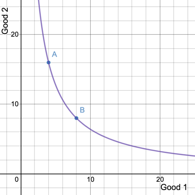
u(x_1,x_2) = x_1x_2
\displaystyle{MU_1 = {\partial u(x_1,x_2) \over \partial x_1} =}
\displaystyle{MU_2 = {\partial u(x_1,x_2) \over \partial x_1} =}
4 \times 16
A = (4,16)
B = (8,8)
8 \times 8
x_2
x_1
\displaystyle{x_2 \over x_1}
= 64
= 64
16
8
4
8
\displaystyle{16 \over 4}
=4
\displaystyle{8 \over 8}
=1
MRS = 4
MRS = 1
Desirable Properties of Preferences
We've asserted that all (rational) preferences are complete and transitive.
There are some additional properties which are true of some preferences:
- Monotonicity
- Convexity
- Continuity
- Smoothness
Monotonic Preferences: “More is Better"
\text{For any bundles }A=(a_1,a_2)\text{ and }B=(b_1,b_2)\text{, }A \succeq B \text{ if } a_1 \ge b_1 \text{ and } a_2 \ge b_2
\text{In other words, all marginal utilities are positive: }MU_1 \ge 0, MU_2 \ge 0
Nonmonotonic Preferences and Satiation
Some goods provide positive marginal utility only up to a point, beyond which consuming more of them actually decreases your utility.
Strict vs. Weak Monotonicity
Strict monotonicity: any increase in any good strictly increases utility (\(MU > 0\) for all goods)
Weak monotonicity: no increase in any good will strictly decrease utility (\(MU \ge 0\) for all goods)
Example: Pfizer's COVID-19 vaccine has a dose of 0.3mL, Moderna's has a dose of 0.5mL
Convex Preferences: “Variety is Better"
Take any two bundles, \(A\) and \(B\), between which you are indifferent.
Would you rather have a convex combination of those two bundles,
than have either of those bundles themselves?
If you would always answer yes, your preferences are convex.
Concave Preferences: “Variety is Worse"
Take any two bundles, \(A\) and \(B\), between which you are indifferent.
Would you rather have a convex combination of those two bundles,
than have either of those bundles themselves?
If you would always answer no, your preferences are concave.
Common Mistakes about Convexity
1. Convexity does not imply you always want equal numbers of things.
2. It's preferences which are convex, not the utility function.
Other Desirable Properties
Continuous: utility functions don't have "jumps"
Smooth: marginal utilities don't have "jumps"
Counter-example: vaccine dose example
Counter-example: Leontief/Perfect Complements utility function
Well-Behaved Preferences
If preferences are strictly monotonic, strictly convex, continuous, and smooth, then:
Indifference curves are smooth, downward-sloping, and bowed in toward the origin
The MRS is diminishing as you move down and to the right along an indifference curve
Good 1 \((x_1)\)
Good 2 \((x_2)\)
"Law of Diminishing MRS"
Summary
MRS(x_1,x_2) = \frac{\partial u(x_1,x_2) \over \partial x_1}{\partial u(x_1,x_2) \over \partial x_2} = {MU_1 \over MU_2}
UNITS OF GOOD 1
UNITS OF GOOD 2
\text{Along the level set }f(x,y)=z,
\displaystyle{{dy \over dx}}
= -
\displaystyle{{\partial f \over \partial x}}
\displaystyle{{\partial f \over \partial y}}
IMPLICIT FUNCTION THEOREM
The Marginal Rate of Substitution is the magnitude of the slope of an indifference curve; so, by the implicit function theorem:
Econ 50 | Spring 25 | Lecture 3
By Chris Makler
Econ 50 | Spring 25 | Lecture 3
Modeling Production with Multivariate Functions


