Computergrafik
Transformationen
Motivation
- Objekte werden mehrfach in einer 3D-Szene verwendet
- verschiedene Positionen (=Koordinaten)
- in unterschiedlichen Größen
- in verschiedenen Orientierungen
- Objekte können sich über die Zeit verändern → Animation


2D-Transformationen
2D-Translation
\hat{\mathbf{p}}
=
\begin{pmatrix}
\hat{x} \\
\hat{y}
\end{pmatrix}
=
\begin{pmatrix}
x + t_x \\
y + t_y
\end{pmatrix}
=
\mathbf{p}
+
\begin{pmatrix}
t_x \\
t_y
\end{pmatrix}
=
\mathbf{p} + \mathbf{t}
x
y
x
y
- Gegeben sei der Punkt \( \mathbf{p} = (x,y)^T \)
- Punkt \( \mathbf{p} \) wird durch eine Translation \( t \) nach \( \hat{\mathbf{p}} =(\hat{x}, \hat{y})^T \) verschoben
2D-Skalierung
\hat{\mathbf{p}}
=
\begin{pmatrix}
s_x\,x \\
s_y\,y
\end{pmatrix}
=
\begin{bmatrix}
s_x & 0 \\
0 & s_y
\end{bmatrix}
\begin{pmatrix}
x \\
y
\end{pmatrix}
\hat{\mathbf{p}}
=
\begin{pmatrix}
s\,x \\
s\,y
\end{pmatrix}
=
s\,\mathbf{p}
x
y
x
y
- Gegeben sei der Punkt \( \mathbf{p} = (x,y)^T \)
- Punkt \( \mathbf{p} \) wird durch eine Skalierung
mit Faktor \( s \) nach \( \hat{\mathbf{p}} =(\hat{x}, \hat{y})^T \) verschoben
2D-Rotation
- Rotationen werden durch Drehung des Koordinatensystems erreicht
- Bei Drehung um einen Winkel \( \alpha \) erhalten wir die Achsen \( b_x \) und \( b_y \) wie folgt:
\mathbf{b_x} = \begin{pmatrix} \cos\,\alpha \\ \sin\,\alpha \end{pmatrix}
\mathbf{b_y} = \begin{pmatrix} -\sin\,\alpha \\ \cos\,\alpha \end{pmatrix}
\alpha
\sin(\alpha)
\cos(\alpha)
\mathbf{b_x}
\mathbf{x}
\mathbf{y}
\mathbf{b_y}
Vereinheitlichung durch Matrizen
\hat{\mathbf{p}}
=
\underbrace{
\begin{bmatrix}
b_x & b_y
\end{bmatrix}
}_{R}
\begin{pmatrix}
x \\
y
\end{pmatrix}
=
\underbrace{
\begin{bmatrix}
\cos\alpha & -\sin\alpha \\
\sin\alpha & \cos\alpha
\end{bmatrix}
}_{R}
\begin{pmatrix}
x \\
y
\end{pmatrix}
=
R\,\mathbf{p}
- Wir können Rotationen auch in Matrix-Schreibweise (\( R \)) ausdrücken:
- Die Skalierung in Matrix-Schreibweise kennen wir bereits:
\hat{\mathbf{p}}
=
\begin{pmatrix}
s_x\,x \\
s_y\,y
\end{pmatrix}
=
\begin{bmatrix}
s_x & 0 \\
0 & s_y
\end{bmatrix}
\begin{pmatrix}
x \\
y
\end{pmatrix}


Und die
Translation?
Homogene Koordinaten
\mathbf{p}
=
\begin{pmatrix}
x\\
y
\end{pmatrix}
\qquad\Longrightarrow\qquad
\underline{\mathbf{p}}
=
\begin{pmatrix}
x\\
y\\
1
\end{pmatrix}
- Wir überführen Punkt \( \mathbf{p} \) in homogene Koordinaten \( \mathbf{\underline{p}} \) wie folgt:
- Damit können wir die Translation wie folgt anpassen:
T
=
\begin{bmatrix}
1 & 0 & t_x\\
0 & 1 & t_y\\
0 & 0 & 1
\end{bmatrix}
T
\underline{\mathbf{p}}
=
\begin{pmatrix}
x+t_x\\
y+t_y\\
1
\end{pmatrix}
Homogene Koordinaten
R
=
\begin{bmatrix}
\cos\alpha & -\sin\alpha & 0\\
\sin\alpha & \cos\alpha & 0\\
0 & 0 & 1
\end{bmatrix}
- Wir passen jetzt die Rotation für homogene Koordinaten an:
- Die Skalierung mit homogene Koordinaten sieht wie folgt aus:
S
=
\begin{bmatrix}
s_x & 0 & 0\\
0 & s_y & 0\\
0 & 0 & 1
\end{bmatrix}
Homogene Koordinaten (alles zusammen)
\mathbf{p}_1
=
S\underline{\mathbf{p}}
\\
\\
\mathbf{p}_2
=
R\mathbf{p}_1
\\
\\
\mathbf{p}_3
=
T\mathbf{p}_2
\\
\\
\mathbf{p}_4
=
TRS\,\underline{\mathbf{p}}
\\
\\
\\
M = TRS
- Skalierung mit \( \mathbf{S} \) → \( \mathbf{p_1} \)
- Rotation mit \( \mathbf{R} \) → \( \mathbf{p_2} \)
- Translation mit \( \mathbf{T} \) → \( \mathbf{p_3} \)
- Wir kombinieren alles in einem Schritt \( \mathbf{TRS} \)→ \( \mathbf{p_4} \)
- \( \mathbf{M} \) fasst \( \mathbf{TRS} \) zusammen
Reihenfolge der Transformationen
Bild: A. Nischwitz
Die Reihenfolge der Transformationen ist wichtig!

3D-Transformationen

3D-Rotation
- Rotationen um die Hauptachsen (Rechtssystem):
R_x(\alpha) = \begin{bmatrix} 1 & 0 & 0 & 0 \\ 0 & \cos\alpha & -\sin\alpha & 0 \\ 0 & \sin\alpha & \cos\alpha & 0 \\ 0 & 0 & 0 & 1 \end{bmatrix} \quad
R_z(\alpha) = \begin{bmatrix} \cos\alpha & -\sin\alpha & 0 & 0 \\ \sin\alpha & \cos\alpha & 0 & 0 \\ 0 & 0 & 1 & 0 \\ 0 & 0 & 0 & 1 \end{bmatrix}
R_y(\alpha) = \begin{bmatrix} \cos\alpha & 0 & \sin\alpha & 0 \\ 0 & 1 & 0 & 0 \\ -\sin\alpha & 0 & \cos\alpha & 0 \\ 0 & 0 & 0 & 1 \end{bmatrix}
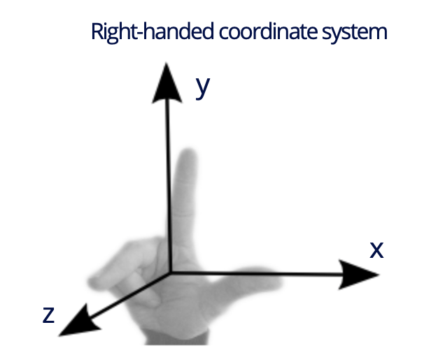
Bild: T. Thormählen
3D-Skalierung und Translation
S(s_x, s_y, s_z) = \begin{bmatrix}
s_x & 0 & 0 & 0 \\
0 & s_y & 0 & 0 \\
0 & 0 & s_z & 0 \\
0 & 0 & 0 & 1
\end{bmatrix}
- Skalierung entlang der Hauptachsen mit Faktoren \( s_x, s_y, s_z \):
T(t_x, t_y, t_z) = \begin{bmatrix}
1 & 0 & 0 & t_x \\
0 & 1 & 0 & t_y \\
0 & 0 & 1 & t_z \\
0 & 0 & 0 & 1
\end{bmatrix}
- Verschiebung um den Vektor \( \mathbf{t} = (t_x, t_y, t_z)^T \):
Perspektivische Projektionen


Bild: D. Jimenez
Perspektivische Projektion
Bild: By SharkD (CC BY-SA 4.0), https://commons.wikimedia.org/w/index.php?curid=58479044, altered by small visibility changes


Bild: G. Mansfield
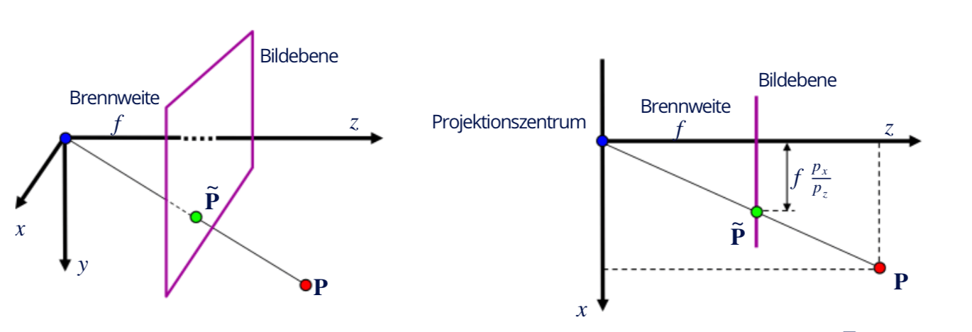
Perspektivische Projektion
Bild: T. Thormählen (adaptiert)
\( \hat{\mathbf{P}} \)
\( \hat{\mathbf{P}} \)
- Wir projizieren einen 3D-Punkt \( \mathbf{P} = (p_x, p_y, p_z)^T \) auf einen Punkt \( \mathbf{\hat{P}} = (\hat{p_x}, \hat{p_y}, \hat{p_z})^T \) auf der Bildebene der Kamera:
\hat{\mathbf{P}} =
\begin{pmatrix}
f \frac{p_x}{p_z}, f \frac{p_y}{p_z}, f
\end{pmatrix}^T
→ siehe Strahlensatz:
\frac{\hat{p}_x}{f} = \frac{p_x}{p_z},
\qquad
\frac{\hat{p}_y}{f} = \frac{p_y}{p_z}
Perspektivische Projektion
\underline{\hat{\mathbf{P}}}
=
\begin{pmatrix}
f p_x \\
f p_y \\
f p_z \\
-p_z
\end{pmatrix}
=
\begin{bmatrix}
f & 0 & 0 & 0 \\
0 & f & 0 & 0 \\
0 & 0 & f & 0 \\
0 & 0 & -1 & 0
\end{bmatrix}
\begin{pmatrix}
f p_x \\
f p_y \\
f p_z \\
1
\end{pmatrix}
\hat{\mathbf{P}}
=
\begin{pmatrix}
\hat{p}_x \\
\hat{p}_y \\
\hat{p}_z
\end{pmatrix}
=
\begin{pmatrix}
f\,\dfrac{p_x}{p_z} \\
f\,\dfrac{p_y}{p_z} \\
f
\end{pmatrix}
\in \mathbb{R}^3
\;\mapsto\;
\underline{\hat{\mathbf{P}}}
=
\begin{pmatrix}
f\,p_x \\
f\,p_y \\
f\,p_z \\
p_z
\end{pmatrix}
\in \mathbb{H}^3
- Wir können es dann wieder als
4x4-Matrix darstellen:
- Wir überführen \( \hat{\mathbf{P}} \) in homogene Koordinaten → \( \hat{\mathbf{\underline{P}}} \) :
Hinweis: In OpenGL zeigt Kamera in negative z-Richtung, daher \( -p_z \)
Clipping Planes (=Schnittebenen)
- Unterscheidung von:
- Near- und
- Far-Clipping-Ebene
- Beide Ebenen verlaufen parallel zur Bildebene
- Ziel:
- Nur Punkte darstellen, deren z-Koordinate innerhalb der Bereiche der Near- bzw. Far-Ebene fallen
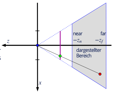
Bild: T. Thormählen
OpenGL: gluLookAt
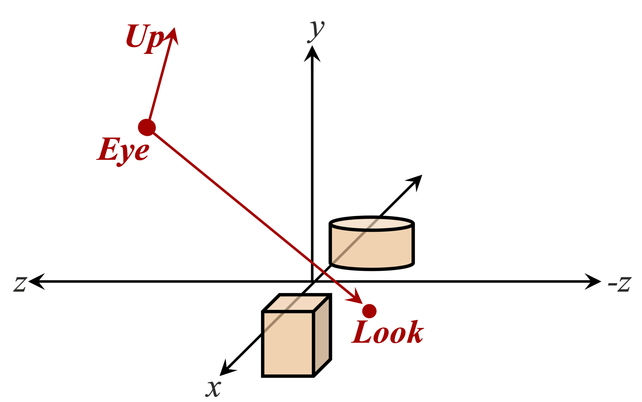
Bild: A. Nischwitz
void gluLookAt(
	// Position der Kamera:
    double eyeX, double eyeY, double eyeZ,
	// Betrachtungspunkt (Look/Center):
    double centerX, double centerY, double centerZ,
	// Up-Vektor (Oben)
    double upX, double upY, double upZ
);
Eye: Wo befindet sich der Betrachter?
Look: Wohin schaut der Betrachter?
Up: Wo ist "Oben"? (meist \( (0, 1, 0) \))
⌨️ Vertex-Shader

Live

coding
✅ Zusammenfassung
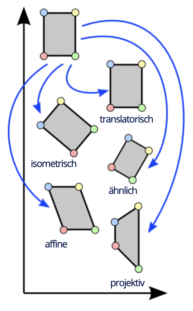
Formen von Transformationen:
- Isometrien: Translation und Rotation
- Ähnlichkeitsabbildung: Translation, Rotation und Skalierung
- Affine Abbildungen: Translation, Rotation, Skalierung und Scherung
- 📸 Projektive Abbildungen: Translation, Rotation, Skalierung, Scherung und Verzerrung
Bild: T. Thormählen
CG6 Transformationen
By blackbill


