Book 1. Market Risk
FRM Part 2
MR 10. Financial Correlation Modeling - Bottom Up Approaches
Presented by: Sudhanshu
Module 1. Financial Correlation Modeling
Module 1. Financial Correlation Modeling
Topic 1. Introduction to Copulas
Topic 2. Copula Functions: Overview
Topic 3. Copula Functions: Expression
Topic 4. Gaussian Copula: Mapping Visualization
Topic 5. Gaussian Copula: Mapping Process
Topic 6. Gaussian Copula: Expression
Topic 7. Applying a Gaussian Copula
Topic 8. Correlated Default Time
Topic 9. Example: Estimating Default Time

Topic 1. Introduction to Copulas
-
Definition: A copula is a joint multivariate distribution that describes how variables from marginal distributions come together.
-
Purpose: Copulas provide a measure of dependence between random variables that is not subject to the same limitations as correlation in applications like risk measurement.
-
Creation: A copula correlation is created by mapping two or more unknown distributions to a known distribution that has well-defined properties.
-
Applications: The Gaussian copula is used to estimate joint probabilities of default for specific time periods and the default time for multiple assets.
Topic 2. Copula Functions: Overview
-
A copula correlation is created by converting two or more unknown distributions that may have unique shapes and mapping them to a known distribution with well-defined properties, such as the normal distribution.
-
Creating a joint probability distribution using a copula:
-
A copula creates a joint probability distribution between two or more variables while maintaining their individual marginal distributions.
-
This is accomplished by mapping multiple distributions to a single multivariate distribution.
-
For example, the following expression defines a copula function, C, that transforms an n-dimensional function on the interval [0,1] to a one-dimensional function.
-
-
The general equation for copula correlation, C, for n variables is defined as:
-
-
-
Where:
-
Gi(ui) are the marginal distributions.
-
C\left[G_1\left(u_1\right), \ldots, G_n\left(u_n\right)\right]=F_n\left[F_1^{-1}\left(G_1\left(u_1\right)\right), \ldots, F_n^{-1}\left(G_n\left(u_n\right)\right) ; \rho_F\right]
C:[0,1]^n \rightarrow[0,1]
-
Suppose is a univariate, uniform distribution with and i ∈ N (i.e., i is an element of set N). A copula function, C, can then be defined as follows:
-
-
Where
-
: joint cumulative distribution function
-
: inverse function of used in the mapping process.
-
: correlation matrix structure of the joint cumulative function
-
-
- Interpretation: A copula function exists that maps the marginal distributions of to via and allows for the joining of the separate values to a single n-variate function that has a correlation matrix of
- Rise in popularity: Copulas gained traction around 2000 for solving complex problems with simple methods
- Key application: Used single multidimensional function to correlate 100+ assets in CDO structures
- Fall from favor: Flexible copula functions lost credibility during 2007–2009 financial crisis
F_1^{-1}
Topic 3. Copula Functions: Expression
G_{\mathrm{i}}\left(u_{\mathrm{i}}\right) \in[0,1]
u_{\mathrm{i}}=u_1, \ldots, u_{\mathrm{n}}
C\left[G_1\left(u_1\right), \ldots, G_n\left(u_n\right)\right]=F_n\left[F_1^{-1}\left(G_1\left(u_1\right)\right), \ldots, F_n^{-1}\left(G_n\left(u_n\right)\right) ; \rho_F\right]
F_n
F_n
\rho_F
F_n
G_1(u_1)
G_n(u_n)
F_1^{-1}G_i(u_i)
F_1^{-1}G_i(u_i)
F_n\left[F_1^{-1}\left(G_1\left(u_1\right)\right), \ldots, F_n^{-1}\left(G_n\left(u_n\right)\right) \right]
\rho_F
Practice Questions: Q1
Q1. Suppose a risk manager creates a copula function, C, defined by the equation:
Which of the following statements does not accurately describe this copula function?
A. are standard normal univariate distributions.
B. is the joint cumulative distribution function.
C. is the inverse function of Fn that is used in the mapping process.
D. is the correlation matrix structure of the joint cumulative function
C\left[G_1\left(u_1\right), \ldots, G_n\left(u_n\right)\right]=F_n\left[F_1^{-1}\left(G_1\left(u_1\right)\right), \ldots, F_n^{-1}\left(G_n\left(u_n\right)\right) ; \rho_F\right]
G_{\mathrm{i}}\left(u_{\mathrm{i}}\right)
F_n
F_1^{-1}
\rho_F
F_n
Practice Questions: Q1 Answer
Explanation: A is correct.
are marginal distributions that do not have well-known distribution properties.
G_{\mathrm{i}}\left(u_{\mathrm{i}}\right)
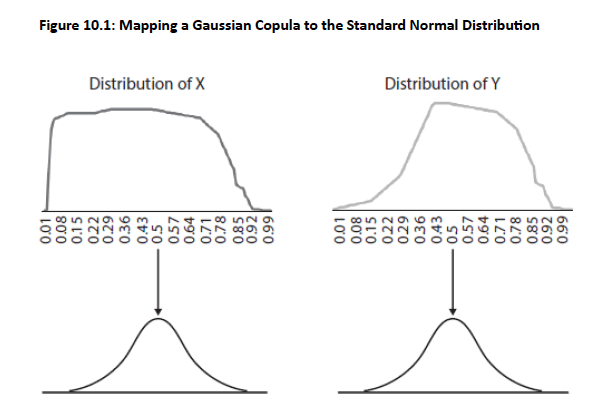
Topic 4. Gaussian Copula: Mapping Visualization
-
The Gaussian copula maps the marginal distribution of each variable to the standard normal distribution.
- Note that the key property of a copula correlation model, including the Gaussian copula, is preserving the original marginal distributions while defining a correlation between them.
-
Figure 10.1 illustrates that the variables of two unknown distributions X and Y have unique marginal distributions.
-
The observations of the unknown distributions are mapped to the standard normal distribution on a percentile-to-percentile basis to create a Gaussian copula.
Topic 5. Gaussian Copula: Mapping Process
- Mapping: Each percentile observation from marginal distribution X (or Y) maps to corresponding percentile on univariate standard normal distribution (e.g., 5th percentile = −1.645)
- Percentile-to-percentile: Transformation applied to every observation in both marginal distributions
- Result: creates multivariate standard normal distribution from original joint distribution
- Purpose: Enables correlation definition between X and Y when original marginal distributions are not well-behaved
- Key advantage: Copulas indirectly define correlation relationships through well-behaved standard normal distributions when direct correlation is difficult to establish
-
The general expression for the Gaussian default time copula for n assets is:
-
-
-
Where:
-
Mn is the joint n-variate standard normal distribution.
-
is the inverse of the univariate standard normal distribution
-
ρM is the correlation matrix structure of the joint standard multivariate normal distribution.
-
The term maps each individual cumulative default probability on a percentile-to-percentile basis to the standard normal distribution.
-
-
In finance, the Gaussian copula is a common approach for measuring default risk. The approach can be transformed to define the Gaussian default time copula, ,in the following expression:
-
- Marginal distributions of cumulative default probabilities, Q(t), for assets i = 1 to n for fixed time periods t are mapped to the single n-variate standard normal distribution Mn with a correlation structure of ρM
-
The term maps each individual cumulative default probability for asset i for time period t on a percentile-to-percentile basis to the standard normal distribution.
-
C_G\left[G_1\left(u_1\right), \ldots, G_n\left(u_n\right)\right]=M_n\left[N_1^{-1}\left(G_1\left(u_1\right)\right), \ldots, N_n^{-1}\left(G_n\left(u_n\right)\right) ; \rho_M\right]
N_1^{-1}
N_1^{-1}(Q_1(t))
Topic 6. Gaussian Copula: Expression
C_{GD}
C_{G D}\left[Q_i(t), \ldots, Q_n(t)\right]=M_n\left[N_1^{-1}\left(Q_1(t)\right), \ldots, N_n^{-1}\left(Q_n(t)\right) ; \rho_M\right]
N_1^{-1}(Q_1(t))
Topic 7. Applying a Gaussian Copula
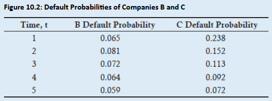
- Example: Suppose a risk manager owns two non-investment grade assets. Figure 10.2 lists the default probabilities for the next five years for Companies B and C that have B and C credit ratings, respectively. How can a Gaussian copula be constructed to estimate the joint default probability, Q, of these two companies in the next year, assuming a one-year Gaussian default correlation of 0.4?
-
Solution: In this example, there are only two companies, B and C. Thus, a bivariate standard normal distribution, ,with a default correlation coefficient of can be applied. With two companies, only a single correlation coefficient is required, and not a correlation matrix of .
-
-
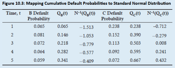
Figure 10.3 illustrates the percentile-to-percentile mapping of cumulative default probabilities for each company to the standard normal distribution.
M_2
\rho_M
\rho
C_{G D}\left[Q_B(t), Q_C(t)\right]=M_2\left[N^{-1}\left(Q_B(t)\right), N^{-1}\left(Q_C(t)\right) ; \rho\right]
Practice Questions: Q2
Q2. Which of the following statements best describes a Gaussian copula?
A. A major disadvantage of a Gaussian copula model is the transformation of the original marginal distributions in order to define the correlation matrix.
B. The mapping of each variable to the new distribution is done by defining a mathematical relationship between marginal and unknown distributions.
C. A Gaussian copula maps the marginal distribution of each variable to the standard normal distribution.
D. A Gaussian copula is seldom used in financial models because ordinal numbers are required.
Practice Questions: Q2 Answer
Explanation: C is correct.
Observations of the unknown marginal distributions are mapped to the standard normal distribution on a percentile-to-percentile basis to create a Gaussian copula.
Practice Questions: Q3
Q3. A Gaussian copula is constructed to estimate the joint default probability of two assets within a one-year time period. Which of the following statements regarding this type of copula is incorrect?
A. This copula requires that the respective cumulative default probabilities are mapped to a bivariate standard normal distribution.
B. This copula defines the relationship between the variables using a default correlation matrix, .
C. The term maps each individual cumulative default probability for asset i for time period t on a percentile-to-percentile basis.
D. This copula is a common approach used in finance to estimate joint default probabilities.
\rho_M
N_1^{-1}\left(Q_1(t)\right)
Practice Questions: Q3 Answer
Explanation: B is correct.
Because there are only two companies, only a single correlation coefficient is required and not a correlation matrix, .
\rho_M
Practice Questions: Q4
Q4. Suppose a risk manager owns two non-investment grade assets and has determined their individual default probabilities for the next five years. Which of the following equations best defines how a Gaussian copula is constructed by the risk manager to estimate the joint probability of these two companies defaulting within the next year, assuming a Gaussian default correlation of 0.35?
A.
B.
C.
D.
\mathrm{C}_{\mathrm{GD}}\left[\mathrm{Q}_{\mathrm{B}}(\mathrm{t}), \mathrm{Q}_{\mathrm{C}}(\mathrm{t})\right]=\mathrm{M}_2\left[\mathrm{~N}^{-1}\left(\mathrm{Q}_{\mathrm{B}}(\mathrm{t})\right), \mathrm{N}^{-1}\left(\mathrm{Q}_{\mathrm{C}}(\mathrm{t})\right) ; \rho\right] .
\mathrm{C}\left[\mathrm{G}_1\left(\mathrm{u}_1\right), \ldots, \mathrm{G}_{\mathrm{n}}\left(\mathrm{u}_{\mathrm{n}}\right)\right]=\mathrm{F}_{\mathrm{n}}\left[\mathrm{~F}_1^{-1}\left(\mathrm{G}_1\left(\mathrm{u}_1\right)\right), \ldots, \mathrm{F}_{\mathrm{n}}^{-1}\left(\mathrm{G}_{\mathrm{n}}\left(\mathrm{u}_{\mathrm{n}}\right)\right) ; \rho_{\mathrm{F}}\right] .
C_{G D}\left[Q_i(t), \ldots, Q_n(t)\right]=M_n\left[N_1^{-1}\left(Q_1(t)\right), \ldots, N_n^{-1}\left(Q_n(t)\right) ; \rho_M\right] .
\mathrm{M}_{\mathrm{n}}(\bullet)=\mathrm{Q}_{\mathrm{i}}\left(\mathrm{\tau}_{\mathrm{i}}\right) .
Practice Questions: Q4 Answer
Explanation: A is correct.
Because there are only two assets, the risk manager should use this equation to define the bivariate standard normal distribution, with a single default correlation coefficient of .
M_2
\rho
Topic 8. Correlated Default Time
-
The Gaussian copula can be used to estimate the default time of an asset correlated to all other assets in a portfolio.
-
The process is summarized as follows:
- Generate a sample: A sample Mn(∙) is derived from a multivariate copula using a Cholesky decomposition when deriving the default time relationship for more than two assets. The sample's default correlations are determined by the default correlation matrix ρM for the n-variate standard normal distribution, Mn
- Equate the sample to cumulative default probability: The sample Mn(∙) is equated to the cumulative individual default probability, Qi(τi), for asset i at time τi using the equation: Mn(∙)=Qi(τi). This is often done using a Newton-Raphson search procedure or Microsoft Excel.
-
Estimate Default Time: The random samples from the n-variate standard normal distribution Mn(∙) are repeatedly drawn (e.g., 100,000 times) to determine the expected default time of asset i. Random samples are drawn to estimate the default times, because there is no closed form solution for this equation.
Topic 9. Example: Estimating Default Time
-
Example: Illustrate how a risk manager estimates the expected default time of asset i using an n-variate Gaussian copula.
-
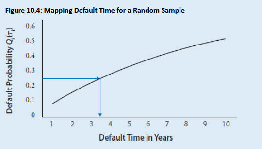
Solution: Suppose a risk manager draws a 25% cumulative default probability for asset i from a random n-variate standard normal distribution, Mn(∙). The n-variate standard normal distribution includes a default correlation matrix, ρM , that has the default correlations of asset i with all n assets. Figure 10.4 illustrates how to equate this 25% with the market determined cumulative individual default probability Qi(τi). Suppose the first random sample equates to a default time τ of 3.5 years. This process is then repeated 100,000 times to estimate the default time of asset i.
Practice Questions: Q5
Q5. A risk manager is trying to estimate the default time for asset i based on the default copula correlation of asset i to n assets. Which of the following equations best defines the process that the risk manager should use to generate and map random samples to estimate the default time?
A.
B.
C.
D.
\mathrm{C}_{\mathrm{GD}}\left[\mathrm{Q}_{\mathrm{B}}(\mathrm{t}), \mathrm{Q}_{\mathrm{C}}(\mathrm{t})\right]=\mathrm{M}_2\left[\mathrm{~N}^{-1}\left(\mathrm{Q}_{\mathrm{B}}(\mathrm{t})\right), \mathrm{N}^{-1}\left(\mathrm{Q}_{\mathrm{C}}(\mathrm{t})\right) ; \rho\right] .
\mathrm{C}\left[\mathrm{G}_1\left(\mathrm{u}_1\right), \ldots, \mathrm{G}_{\mathrm{n}}\left(\mathrm{u}_{\mathrm{n}}\right)\right]=\mathrm{F}_{\mathrm{n}}\left[\mathrm{~F}_1^{-1}\left(\mathrm{G}_1\left(\mathrm{u}_1\right)\right), \ldots, \mathrm{F}_{\mathrm{n}}^{-1}\left(\mathrm{G}_{\mathrm{n}}\left(\mathrm{u}_{\mathrm{n}}\right)\right) ; \rho_{\mathrm{F}}\right] .
C_{G D}\left[Q_i(t), \ldots, Q_n(t)\right]=M_n\left[N_1^{-1}\left(Q_1(t)\right), \ldots, N_n^{-1}\left(Q_n(t)\right) ; \rho_M\right] .
\mathrm{M}_{\mathrm{n}}(\bullet)=\mathrm{Q}_{\mathrm{i}}\left(\mathrm{\tau}_{\mathrm{i}}\right) .
Practice Questions: Q5 Answer
Explanation: D is correct.
The equation is used to repeatedly generate random drawings from the n-variate standard normal distribution to determine the expected default time using the Gaussian copula.
\mathrm{M}_{\mathrm{n}}(\bullet)=\mathrm{Q}_{\mathrm{i}}\left(\mathrm{\tau}_{\mathrm{i}}\right)
Copy of MR 10. Financial Correlation Modeling-Bottom up Approaches
By Prateek Yadav


