Cinemática de robots de base flotante, fuerzas de contacto y el modelo de fricción de Coulomb
MT3005 - Robótica 1

Un nuevo tipo de robot
el jacobiano nos brindó una forma de hablar sobre las fuerzas a las que se encuentra sometido el efector final de un manipulador
el jacobiano nos brindó una forma de hablar sobre las fuerzas a las que se encuentra sometido el efector final de un manipulador
el hablar de fuerzas nos permite, más allá de la manipulación, considerar un nuevo tipo de robot de alta relevancia en la actualidad
el jacobiano nos brindó una forma de hablar sobre las fuerzas a las que se encuentra sometido el efector final de un manipulador
el hablar de fuerzas nos permite, más allá de la manipulación, considerar un nuevo tipo de robot de alta relevancia en la actualidad
\(\Rightarrow\) robots de base flotante
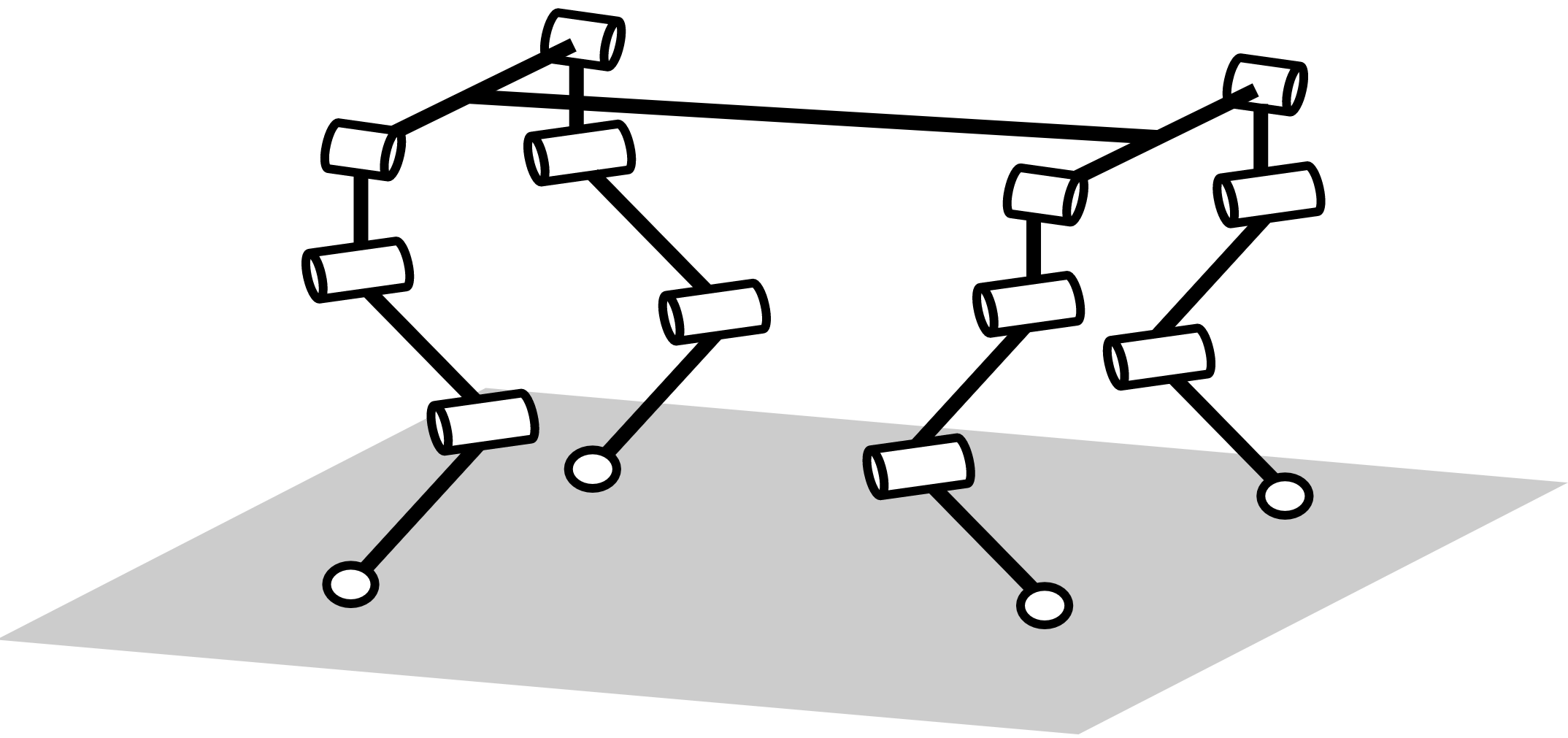
Robots de base flotante
\{B\}
base flotante
(no actuada)
\mathbf{q}_b \in \mathbb{R}^3 \times SO(3)
Robots de base flotante
\{B\}
base flotante
(no actuada)
\mathbf{q}_b \in \mathbb{R}^3 \times SO(3)
depende de la representación para la orientación
Robots de base flotante
\{B\}
\{I\}
base flotante
(no actuada)
\mathbf{q}_b \in \mathbb{R}^3 \times SO(3)
Robots de base flotante
\{B\}
\{I\}
base flotante
(no actuada)
\mathbf{q}_b \in \mathbb{R}^3 \times SO(3)
Robots de base flotante
\{B\}
\{I\}
base flotante
(no actuada)
\mathbf{q}_b \in \mathbb{R}^3 \times SO(3)
Robots de base flotante
\{B\}
\{I\}
base flotante
(no actuada)
grados de libertad virtuales
\mathbf{q}_b \in \mathbb{R}^3 \times SO(3)
Robots de base flotante
\{B\}
\{I\}
base flotante
(no actuada)
manipulador(es) serial(es) (actuados)
grados de libertad virtuales
\mathbf{q}_b \in \mathbb{R}^3 \times SO(3)
\mathbf{q}_j \in \mathcal{C}_1 \times \mathcal{C}_2 \times \cdots
Robots de base flotante
\{B\}
\{I\}
base flotante
(no actuada)
manipulador(es) serial(es) (actuados)
grados de libertad virtuales
fuerzas (restricciones) de contacto
\mathbf{q}_b \in \mathbb{R}^3 \times SO(3)
\mathbf{q}_j \in \mathcal{C}_1 \times \mathcal{C}_2 \times \cdots
Robots de base flotante
\{B\}
\{I\}
{^I}\mathbf{T}_B\left(\mathbf{q}_b\right)
Cinemática directa (de la base)
\{B\}
\{I\}
{^I}\mathbf{T}_B\left(\mathbf{q}_b\right)
\mathbf{q}_b=\begin{bmatrix} \mathbf{q}_{b_P} \\ \mathbf{q}_{b_O} \end{bmatrix}
\dim\left(\mathbf{q}_{b_P}\right) = 3
\min\left(\dim\left(\mathbf{q}_{b_O}\right)\right) = 3
n_b=\dim\left(\mathbf{q}_b\right)
Cinemática directa (de la base)
\{B\}
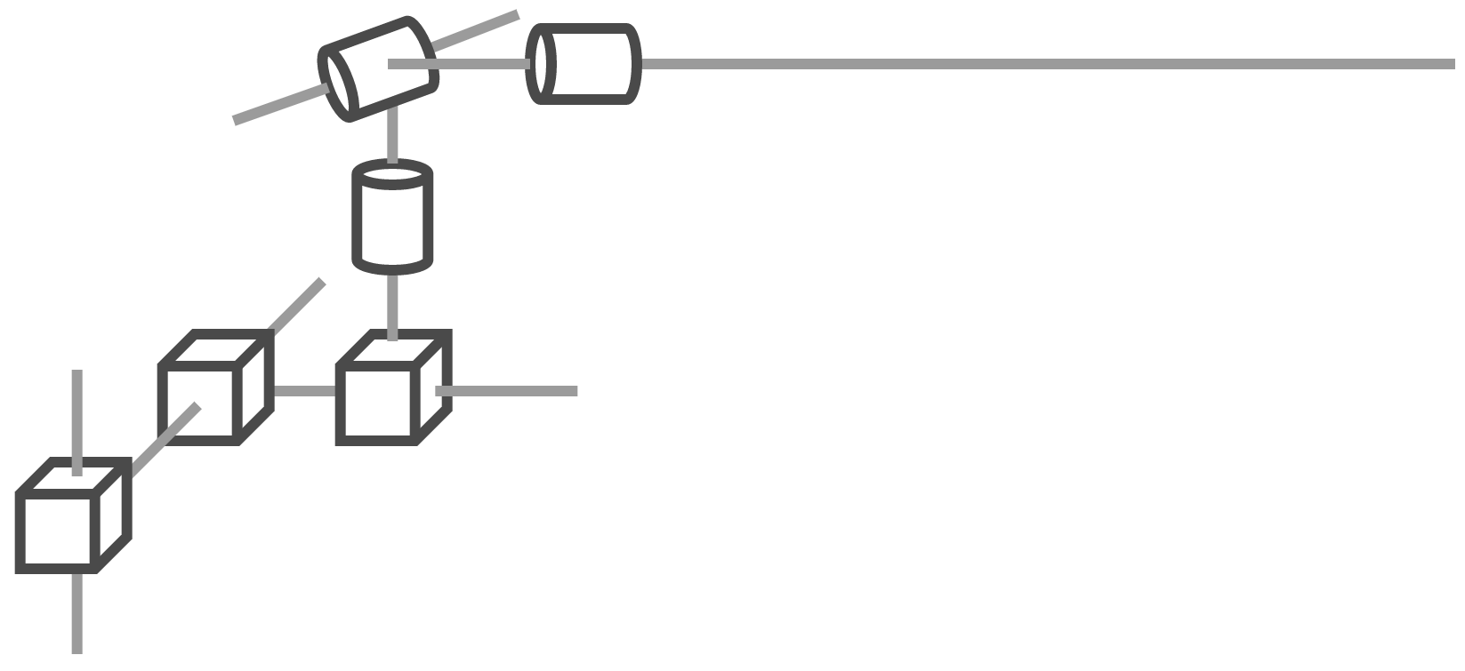
Cinemática directa (de las patas)
\{B\}
\{B_1\}
\{E_1\}
Cinemática directa (de las patas)
\{B\}
\{B_1\}
\{E_1\}
\mathcal{K}_1\left(\mathbf{q}_{j_1}\right) \subseteq {^{B_1}}\mathbf{T}_{E_1}\left(\mathbf{q}_{j_1}\right)
{^B}\mathbf{T}_{E_1}\left(\mathbf{q}_{j_1}\right)={^B}\mathbf{T}_{B_1}\mathcal{K}_1\left(\mathbf{q}_{j_1}\right)
Cinemática directa (de las patas)
\{B\}
\{B_1\}
\{E_1\}
\mathcal{K}_1\left(\mathbf{q}_{j_1}\right) \subseteq {^{B_1}}\mathbf{T}_{E_1}\left(\mathbf{q}_{j_1}\right)
{^B}\mathbf{T}_{E_1}\left(\mathbf{q}_{j_1}\right)={^B}\mathbf{T}_{B_1}\mathcal{K}_1\left(\mathbf{q}_{j_1}\right)
\Rightarrow {^I}\mathbf{T}_{E_1}\left(\mathbf{q}\right)={^I}\mathbf{T}_B\left(\mathbf{q}_b\right){^B}\mathbf{T}_{E_1}\left(\mathbf{q}_{j_1}\right)
\mathbf{q}=\begin{bmatrix} \mathbf{q}_b \\ \mathbf{q}_j \end{bmatrix}
n_j=\dim\left(\mathbf{q}_j\right)
Cinemática directa (de las patas)
\{B\}
\{B_1\}
\{E_1\}
\mathcal{K}_1\left(\mathbf{q}_{j_1}\right) \subseteq {^{B_1}}\mathbf{T}_{E_1}\left(\mathbf{q}_{j_1}\right)
{^B}\mathbf{T}_{E_1}\left(\mathbf{q}_{j_1}\right)={^B}\mathbf{T}_{B_1}\mathcal{K}_1\left(\mathbf{q}_{j_1}\right)
\Rightarrow {^I}\mathbf{T}_{E_1}\left(\mathbf{q}\right)={^I}\mathbf{T}_B\left(\mathbf{q}_b\right){^B}\mathbf{T}_{E_1}\left(\mathbf{q}_j\right)
\mathbf{q}=\begin{bmatrix} \mathbf{q}_b \\ \mathbf{q}_j \end{bmatrix}
n_j=\dim\left(\mathbf{q}_j\right)
Cinemática directa (de las patas)
{^I}\boldsymbol{\mathcal{V}}_{E_1}={^I}\mathbf{J}_1\left(\mathbf{q}\right)\mathbf{v}=
\begin{bmatrix} {^I}\mathbf{J}_{v_1}\left(\mathbf{q}\right) \\ {^I}\mathbf{J}_{\omega_1}\left(\mathbf{q}\right) \end{bmatrix}
\begin{bmatrix} {^I}\mathbf{v}_B \\ {^I}\boldsymbol{\omega}_{IB} \\ \dot{\mathbf{q}}_j \end{bmatrix}
Cinemática diferencial
{^I}\boldsymbol{\mathcal{V}}_{E_1}={^I}\mathbf{J}_1\left(\mathbf{q}\right)\mathbf{v}=
\begin{bmatrix} {^I}\mathbf{J}_{v_1}\left(\mathbf{q}\right) \\ {^I}\mathbf{J}_{\omega_1}\left(\mathbf{q}\right) \end{bmatrix}
\begin{bmatrix} {^I}\mathbf{v}_B \\ {^I}\boldsymbol{\omega}_{IB} \\ \dot{\mathbf{q}}_j \end{bmatrix}
velocidad generalizada
\dim\left(\dot{\mathbf{q}}_{b_O}\right) \stackrel{?}{=} \dim\left({^I}\boldsymbol{\omega}_{IB}\right)
Cinemática diferencial
{^I}\boldsymbol{\mathcal{V}}_{E_1}={^I}\mathbf{J}_1\left(\mathbf{q}\right)\mathbf{v}=
\begin{bmatrix} {^I}\mathbf{J}_{v_1}\left(\mathbf{q}\right) \\ {^I}\mathbf{J}_{\omega_1}\left(\mathbf{q}\right) \end{bmatrix}
\begin{bmatrix} {^I}\mathbf{v}_B \\ {^I}\boldsymbol{\omega}_{IB} \\ \dot{\mathbf{q}}_j \end{bmatrix}
\mathbf{E}_{\chi_R} \dot{\mathbf{q}}_{b_O}
transformación (jacobiano) entre la velocidad de la representación de orientación a las rotaciones alrededor de los ejes
velocidad generalizada
\dim\left(\dot{\mathbf{q}}_{b_O}\right) \stackrel{?}{=} \dim\left({^I}\boldsymbol{\omega}_{IB}\right)
Cinemática diferencial
\dot{\mathbf{q}}_{b_P}
{^I}\mathbf{J}_1\left(\mathbf{q}\right)=\begin{bmatrix} \mathbf{I}_{3 \times 3} & -{^I}\mathbf{R}_{B}\left(\mathbf{q}_b\right)\mathcal{S}\left({^B}\mathbf{o}_{E_1}\right) & {^I}\mathbf{R}_{B}\left(\mathbf{q}_b\right){^B}\mathbf{J}_{v_1}\left(\mathbf{q}_j\right) \\
\mathbf{0}_{3 \times 3} & {^I}\mathbf{R}_{B}\left(\mathbf{q}_b\right) & {^I}\mathbf{R}_{B}\left(\mathbf{q}_b\right){^B}\mathbf{J}_{\omega_1}\left(\mathbf{q}_j\right) \end{bmatrix}
{^I}\boldsymbol{\mathcal{V}}_{E_1}={^I}\mathbf{J}_1\left(\mathbf{q}\right)\mathbf{v}=
\begin{bmatrix} {^I}\mathbf{J}_{v_1}\left(\mathbf{q}\right) \\ {^I}\mathbf{J}_{\omega_1}\left(\mathbf{q}\right) \end{bmatrix}
\begin{bmatrix} {^I}\mathbf{v}_B \\ {^I}\boldsymbol{\omega}_{IB} \\ \dot{\mathbf{q}}_j \end{bmatrix}
\mathbf{E}_{\chi_R} \dot{\mathbf{q}}_{b_O}
transformación (jacobiano) entre la velocidad de la representación de orientación a las rotaciones alrededor de los ejes
velocidad generalizada
\dim\left(\dot{\mathbf{q}}_{b_O}\right) \stackrel{?}{=} \dim\left({^I}\boldsymbol{\omega}_{IB}\right)
Cinemática diferencial
\dot{\mathbf{q}}_{b_P}
\mathbf{E}_{R,\mathrm{eulerXYZ}}=\begin{bmatrix} 1 & 0 & \sin(\theta_y) \\
0 & \cos(\theta_x) & -\cos(\theta_y)\sin(\theta_x) \\
0 & \sin(\theta_x) & \cos(\theta_x)\cos(\theta_y) \end{bmatrix}
\mathbf{E}_{R,\mathrm{quat}}=2\mathbf{H}\left(\boldsymbol{\mathcal{Q}}\right), \qquad \mathbf{H}\left(\boldsymbol{\mathcal{Q}}\right)=
\begin{bmatrix} -\epsilon_1 & \eta & -\epsilon_3 & \epsilon_2 \\
-\epsilon_2 & \epsilon_3 & \eta & -\epsilon_1 \\
-\epsilon_3 & -\epsilon_2 & \epsilon_1 & \eta \end{bmatrix}
Ejemplos de mapeos entre velocidades
¿Contactos?
dado que no podemos actuar la base flotante de forma directa, es necesario actuarla indirectamente mediante fuerzas externas que resultan de contactos
¿Contactos?
dado que no podemos actuar la base flotante de forma directa, es necesario actuarla indirectamente mediante fuerzas externas que resultan de contactos
¿Cómo caracterizamos estos contactos?
¿Contactos?
Fuerzas (restricciones) de contacto
en el punto de contacto:
{^B}\mathbf{o}_{E_1}(\mathbf{q}_{j_1})=\mathbf{0}
\to \mathbf{h}\left(\mathbf{q}\right)=\mathbf{0}
restricción bilateral de posición
Fuerzas (restricciones) de contacto
en el punto de contacto:
{^B}\mathbf{o}_{E_1}(\mathbf{q}_{j_1})=\mathbf{0}
\to \mathbf{h}\left(\mathbf{q}\right)=\mathbf{0}
\dot{\mathbf{h}}\left(\mathbf{q}\right)=\mathbf{H}\left(\mathbf{q}\right)\dot{\mathbf{q}}=\mathbf{0}
restricción bilateral de posición
velocidad:
Fuerzas (restricciones) de contacto
en el punto de contacto:
jacobiano de restricción
{^B}\mathbf{o}_{E_1}(\mathbf{q}_{j_1})=\mathbf{0}
\to \mathbf{h}\left(\mathbf{q}\right)=\mathbf{0}
\dot{\mathbf{h}}\left(\mathbf{q}\right)=\mathbf{H}\left(\mathbf{q}\right)\dot{\mathbf{q}}=\mathbf{0}
restricción bilateral de posición
velocidad:
Fuerzas (restricciones) de contacto
en el punto de contacto:
restricción de Pfaffian
{^B}\mathbf{o}_{E_1}(\mathbf{q}_{j_1})=\mathbf{0}
\to \mathbf{h}\left(\mathbf{q}\right)=\mathbf{0}
\dot{\mathbf{h}}\left(\mathbf{q}\right)=\mathbf{H}\left(\mathbf{q}\right)\dot{\mathbf{q}}=\mathbf{0}
\ddot{\mathbf{h}}\left(\mathbf{q}\right)=\mathbf{H}\left(\mathbf{q}\right)\ddot{\mathbf{q}}+\dot{\mathbf{H}}\left(\mathbf{q},\dot{\mathbf{q}}\right)\dot{\mathbf{q}}=\mathbf{0}
restricción bilateral de posición
velocidad:
aceleración:
Fuerzas (restricciones) de contacto
en el punto de contacto:
estas restricciones son suficientes si no consideramos fricción
desafortunadamente, debemos consderar fricción para considerar casos realistas
Fuerzas (restricciones) de contacto
El modelo de fricción de Coulomb
m
f_n
f_t
f
x
v=\dot{x}
m
f_n
f_t
f
x
v=\dot{x}
\(f_n\) mantiene "pegada" la masa al suelo
m
f_n
f_t
f
x
v=\dot{x}
\(f_n\) mantiene "pegada" la masa al suelo
si \(f\) es suficientemente grande, la masa comienza a moverse
f_t
v
\mu f_n
-\mu f_n
v=0: \quad \|f_t\| \le \mu f_n
v\ne 0: \quad f_t= -\mu f_n \dfrac{v}{\|v\|}
v= 0, a\ne 0: \quad f_t= -\mu f_n \dfrac{a}{\|a\|}
f_t
v
\mu f_n
-\mu f_n
v=0: \quad \|f_t\| \le \mu f_n
v\ne 0: \quad f_t= -\mu f_n \dfrac{v}{\|v\|}
v= 0, a\ne 0: \quad f_t= -\mu f_n \dfrac{a}{\|a\|}
coeficiente de fricción
f_t
v
\mu f_n
-\mu f_n
un mejor modelo es el que típicamente se usa en física fundamental
un mejor modelo es el que típicamente se usa en física fundamental
\mu_s > \mu_k
f_t
v
\mu_k f_n
-\mu_k f_n
-\mu_s f_n
\mu_s f_n
un mejor modelo es el que típicamente se usa en física fundamental
\mu_s > \mu_k
fricción estática
fricción dinámica
f_t
v
\mu_k f_n
-\mu_k f_n
-\mu_s f_n
\mu_s f_n
un mejor modelo es el que típicamente se usa en física fundamental
\mu_s > \mu_k
nos interesa el comportamiento estático
fricción estática
fricción dinámica
\(\to\) esta región, en 3D, se ve como un cono de fricción
f_t
v
\mu_k f_n
-\mu_k f_n
-\mu_s f_n
\mu_s f_n
x\to t_1
y\to t_2
z\to n
x\to t_1
y\to t_2
z\to n
x\to t_1
y\to t_2
z\to n
\mathbf{f}
x\to t_1
y\to t_2
z\to n
cono de fricción
\mathbf{f}
x\to t_1
y\to t_2
z\to n
cono de fricción
\mathcal{FC}=\left\{\mathbf{f} \ | \ f_z\ge 0, \ \sqrt{f_x^2+f_y^2}\le \mu f_z\right\}
\mathbf{f}
x\to t_1
y\to t_2
z\to n
cono de fricción
\mathcal{FC}=\left\{\mathbf{f} \ | \ f_z\ge 0, \ \sqrt{f_x^2+f_y^2}\le \mu f_z\right\}
\mathbf{f}
x\to t_1
y\to t_2
z\to n
cono de fricción
\mathcal{FC}=\left\{\mathbf{f} \ | \ f_z\ge 0, \ \sqrt{f_x^2+f_y^2}\le \mu f_z\right\}
\mathbf{f}
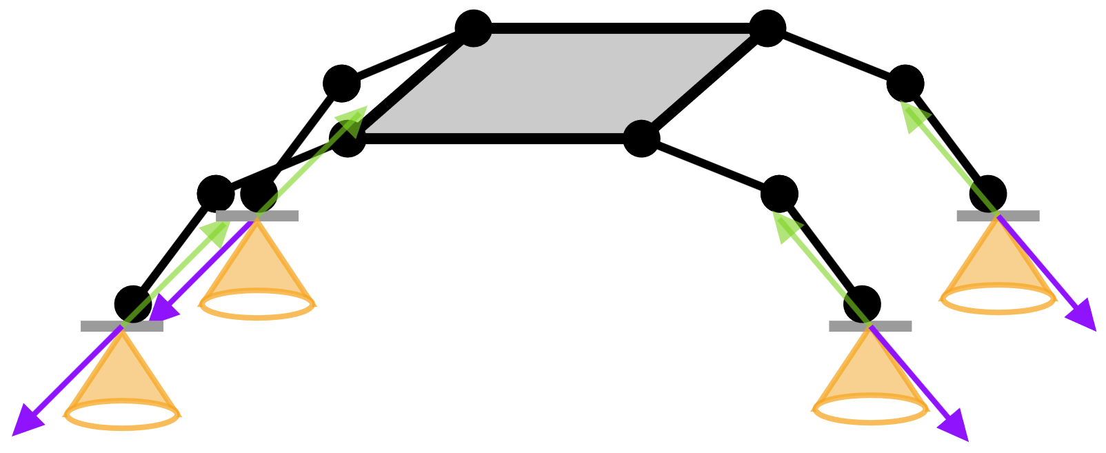
\(\Rightarrow \mathbf{f}\in\mathcal{FC}\) para que no haya deslizamiento
entonces, las fuerzas de contacto deben mantenerse dentro de los conos de fricción para que no haya deslizamiento
Contacto sin deslizamiento
entonces, las fuerzas de contacto deben mantenerse dentro de los conos de fricción para que no haya deslizamiento
Contacto sin deslizamiento
sin deslizamiento
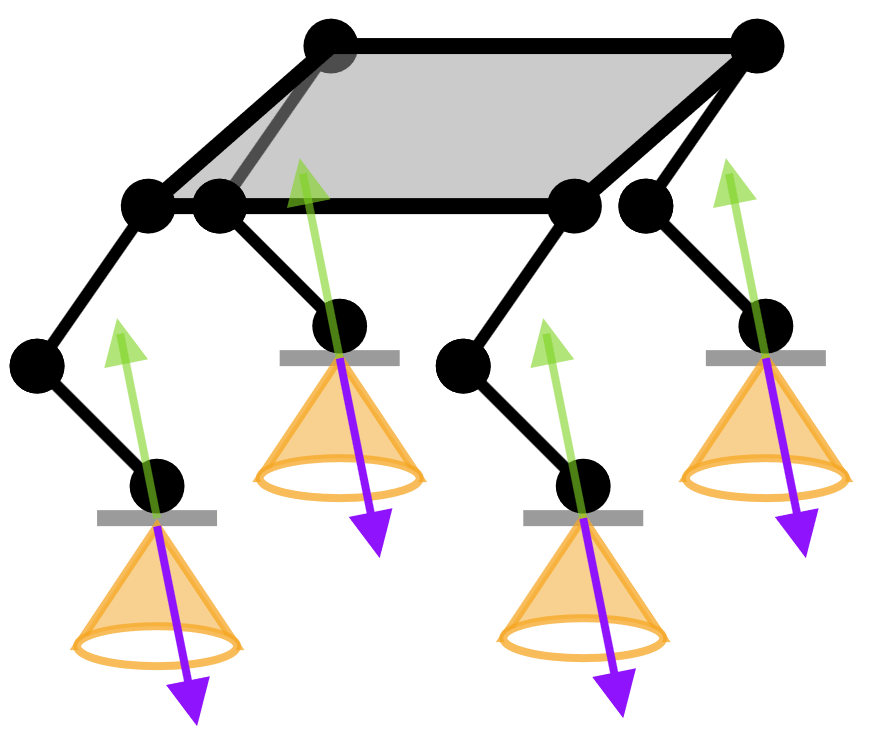
entonces, las fuerzas de contacto deben mantenerse dentro de los conos de fricción para que no haya deslizamiento
Contacto sin deslizamiento
sin deslizamiento
con deslizamiento
Referencias
- ETH Zürich - Robot Dynamics Lecture Notes 2019.pdf
MT3005 - Lecture 8 (2025)
By Miguel Enrique Zea Arenales


