Control de robots móviles con ruedas
MT3005 - Robótica 1

Partiendo del robot diferencial
{^I}\dot{\boldsymbol{\xi}}=\dfrac{r}{2}\begin{bmatrix} \cos\theta & \cos\theta \\ \sin\theta & \sin\theta \\ 1/\ell & -1/\ell \end{bmatrix}
\begin{bmatrix} \dot{\varphi}_R \\ \dot{\varphi}_L \end{bmatrix}
\ell
\ell
r
v_r
v_\ell
\dot{x}=\dfrac{r\left(\dot{\varphi}_R+\dot{\varphi}_L\right)}{2}\cos\theta
\dot{y}=\dfrac{r\left(\dot{\varphi}_R+\dot{\varphi}_L\right)}{2}\sin\theta
\dot{\theta}=\dfrac{r\left(\dot{\varphi}_R-\dot{\varphi}_L\right)}{2\ell}
ya con el modelo del robot procedamos a controlarlo
sistema dinámico simple pero que presenta un comportamiento representativo del sistema completo
modelo de orden reducido (template)
Otra arquitectura jerárquica de control
sistema completo con actuadores ideales
referencias
sistema dinámico simple pero que presenta un comportamiento representativo del sistema completo
sistema dinámico como convencionalmente lo conocemos
modelo de orden reducido (template)
Otra arquitectura jerárquica de control
sistema completo con actuadores ideales
actuadores reales
referencias
referencias
servomecanismos a bajo nivel
(control clásico)
sistema dinámico simple pero que presenta un comportamiento representativo del sistema completo
(control moderno | IA )
sistema dinámico como convencionalmente lo conocemos
(control moderno)
modelo de orden reducido (template)
Otra arquitectura jerárquica de control
Otra arquitectura jerárquica de control
sistema completo con actuadores ideales
actuadores reales
referencias
referencias
servomecanismos a bajo nivel
(control clásico)
sistema dinámico simple pero que presenta un comportamiento representativo del sistema completo
(control moderno | IA )
sistema dinámico como convencionalmente lo conocemos
(control moderno)
modelo de orden reducido (template)
¿Por qué no emplear control convencional?
el comportamiento no holonómico de la mayoría de robots móviles con ruedas genera dificultades para el control
el comportamiento no holonómico de la mayoría de robots móviles con ruedas genera dificultades para el control
por ejemplo, ¿Qué pasa si tratamos de aplicar control LTI directamente?
el comportamiento no holonómico de la mayoría de robots móviles con ruedas genera dificultades para el control
por ejemplo, ¿Qué pasa si tratamos de aplicar control LTI directamente?
\mathbf{f}\left({^I}\boldsymbol{\xi}_{ss},\mathbf{v}_{ss}\right)=\mathbf{0}
el comportamiento no holonómico de la mayoría de robots móviles con ruedas genera dificultades para el control
por ejemplo, ¿Qué pasa si tratamos de aplicar control LTI directamente?
\mathbf{f}\left({^I}\boldsymbol{\xi}_{ss},\mathbf{v}_{ss}\right)=\mathbf{0}
{^I}\boldsymbol{\xi}_{ss}=\begin{bmatrix} x_{ss} & y_{ss} & \theta_{ss} \end{bmatrix}^\top \\
\mathbf{v}_{ss}=\mathbf{0}
\begin{cases}
\dot{\mathbf{z}}=\mathbf{A}\mathbf{z}+\mathbf{B}\boldsymbol{\mu} \\
\mathbf{w}=\mathbf{C}\mathbf{z}
\end{cases}
{^I}\boldsymbol{\xi}_{ss}=\begin{bmatrix} x_{ss} & y_{ss} & \theta_{ss} \end{bmatrix}^\top \\
\mathbf{v}_{ss}=\mathbf{0}
\begin{cases}
\dot{\mathbf{z}}=\mathbf{A}\mathbf{z}+\mathbf{B}\boldsymbol{\mu} \\
\mathbf{w}=\mathbf{C}\mathbf{z}
\end{cases}
{^I}\boldsymbol{\xi}_{ss}=\begin{bmatrix} x_{ss} & y_{ss} & \theta_{ss} \end{bmatrix}^\top \\
\mathbf{v}_{ss}=\mathbf{0}
¿Problema?
el sistema linealizado nunca resulta completamente controlable
\(\Rightarrow\) no pueden emplearse de forma directa los métodos convencionales
modelo uniciclo*
(o boid)
modelo cinemático del robot móvil
motores con ruedas
controlados mediante PIDs (típicamente) de velocidad
el modelo más simple que representa el comportamiento no holonómico de los robots con ruedas (y otros)
derivado con la metodología de la clase anterior
v_\mathrm{ref}, \omega_\mathrm{ref}
\dot{\varphi}_{R,\mathrm{ref}}, \dot{\varphi}_{L,\mathrm{ref}}
Regresando a la arquitectura jerárquica
(x,y)
\theta
El modelo uniciclo
(x,y)
\theta
v
\omega
El modelo uniciclo
\dot{x}=v\cos\theta \\
\dot{y}=v\sin\theta \\
\dot{\theta}=\omega
(x,y)
\theta
v
\omega
El modelo uniciclo
\begin{bmatrix} \dot{x} \\ \dot{y} \\ \dot{\theta} \end{bmatrix} =
\begin{bmatrix} \cos\theta & 0 \\ \sin\theta & 0 \\ 0 & 1 \end{bmatrix} \begin{bmatrix} v \\ \omega \end{bmatrix}
(x,y)
\theta
v
\omega
El modelo uniciclo
\begin{bmatrix} \dot{x} \\ \dot{y} \\ \dot{\theta} \end{bmatrix} =
\begin{bmatrix} \cos\theta & 0 \\ \sin\theta & 0 \\ 0 & 1 \end{bmatrix} \begin{bmatrix} v \\ \omega \end{bmatrix}
(x,y)
\theta
v
\omega
El modelo uniciclo
\mathbf{J}\left({^I}\boldsymbol{\xi}\right)
{^I}\dot{\boldsymbol{\xi}}
\mathbf{v}
\begin{bmatrix} \dot{x} \\ \dot{y} \\ \dot{\theta} \end{bmatrix} =
\begin{bmatrix} \cos\theta & 0 \\ \sin\theta & 0 \\ 0 & 1 \end{bmatrix} \begin{bmatrix} v \\ \omega \end{bmatrix}
(x,y)
\theta
v
\omega
El modelo uniciclo
\mathbf{v}
este modelo aplica para cualquier sistema capaz de moverse hacia adelante y cambiar su dirección
\mathbf{J}\left({^I}\boldsymbol{\xi}\right)
{^I}\dot{\boldsymbol{\xi}}
El modelo uniciclo
- control clásico (posición)
- PID
- PID con acercamiento exponencial
- control moderno LTI (posición)
- LQR
- LQI
- control no lineal (pose)
Controlando al uniciclo
Directamente, mediante el sistema no holonómico (no lineal):
-
PID planteado de forma "ingenua" (punto a punto).
- Modificación de velocidad lineal con acercamiento exponencial.
- Trayectorias mediante pure pursuit y con términos de feedforward.
- Planteamientos basados en Lyapunov.
Controlando al uniciclo
Controlando al uniciclo
Indirectamente, mediante linealización por difeomorfismo:
- PIDs desacoplados (ej: control BART - Tarea IE3036).
- LQR (punto a punto) y LQI (trayectorias).
- Entre otras metodologías de control lineal.
Controlando al uniciclo
Indirectamente, mediante linealización por difeomorfismo:
- PIDs desacoplados (ej: control BART - Tarea IE3036).
- LQR (punto a punto) y LQI (trayectorias).
- Entre otras metodologías de control lineal.
NOTA: las opciones presentadas NO son exhaustivas ya que ni siquiera estamos considerando las estrategias de control típicas en el área de vehículos autónomos.
(x,y)
\theta
(x_g,y_g)
PID de forma ingenua
(x,y)
\theta
(x_g,y_g)
PID de forma ingenua
\theta_g=\arctan\left(\dfrac{y_g-y}{x_g-x}\right)
(x,y)
\theta
(x_g,y_g)
x_g-x
y_g-y
\theta_g
PID de forma ingenua
e_p=\left\| \begin{bmatrix} x_g-x \\ y_g-y \end{bmatrix} \right\|_2
\theta_g=\arctan\left(\dfrac{y_g-y}{x_g-x}\right)
(x,y)
\theta
(x_g,y_g)
x_g-x
y_g-y
\theta_g
e_p
PID de forma ingenua
e_p=\left\| \begin{bmatrix} x_g-x \\ y_g-y \end{bmatrix} \right\|_2
\theta_g=\arctan\left(\dfrac{y_g-y}{x_g-x}\right)
(x,y)
\theta
(x_g,y_g)
x_g-x
y_g-y
\theta_g
e_o
e_p
e_o=\theta_g-\theta
PID de forma ingenua
e_p=\left\| \begin{bmatrix} x_g-x \\ y_g-y \end{bmatrix} \right\|_2
\theta_g=\arctan\left(\dfrac{y_g-y}{x_g-x}\right)
(x,y)
\theta
(x_g,y_g)
x_g-x
y_g-y
\theta_g
e_o
e_p
e_o=\theta_g-\theta
PID de forma ingenua
PROBLEMA
e_p=\left\| \begin{bmatrix} x_g-x \\ y_g-y \end{bmatrix} \right\|_2
\theta_g=\arctan\left(\dfrac{y_g-y}{x_g-x}\right)
(x,y)
\theta
(x_g,y_g)
x_g-x
y_g-y
\theta_g
e_o
e_p
PID de forma ingenua
e_o=\mathrm{atan2}\left(\dfrac{\sin(\theta_g-\theta)}{\cos(\theta_g-\theta)}\right)
e_p=\left\| \begin{bmatrix} x_g-x \\ y_g-y \end{bmatrix} \right\|_2
\theta_g=\arctan\left(\dfrac{y_g-y}{x_g-x}\right)
(x,y)
\theta
(x_g,y_g)
x_g-x
y_g-y
\theta_g
e_o
e_p
PID de forma ingenua
eO = angdiff(theta, theta_g)v = \mathrm{PID}(e_p)=k_{Pp}e_p + k_{Ip}\displaystyle\int_{0}^{t} e_p(\tau)d\tau + k_{Dp}\dot{e}_p \\
\omega = \mathrm{PID}(e_o)=k_{Po}e_o + k_{Io}\displaystyle\int_{0}^{t} e_o(\tau)d\tau + k_{Do}\dot{e}_o
PIDs de posición y orientación
v = \mathrm{PID}(e_p)=k_{Pp}e_p + k_{Ip}\displaystyle\int_{0}^{t} e_p(\tau)d\tau + k_{Dp}\dot{e}_p \\
\omega = \mathrm{PID}(e_o)=k_{Po}e_o + k_{Io}\displaystyle\int_{0}^{t} e_o(\tau)d\tau + k_{Do}\dot{e}_o
este esquema desacopla la posición de la orientación y las controla por separado
\(\Rightarrow\) la convergencia se da en forma de espirales
PIDs de posición y orientación
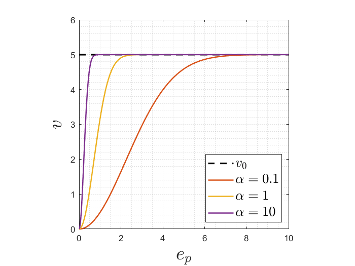
un problema que presenta el PID para la velocidad lineal es que el robot desacelera exponencialmente conforme se acerca a la meta, presentando una convergencia lenta
Acercamiento exponencial
un problema que presenta el PID para la velocidad lineal es que el robot desacelera exponencialmente conforme se acerca a la meta, presentando una convergencia lenta
Acercamiento exponencial
esto puede corregirse (hasta cierto punto) mediante una no linealidad que normalice la velocidad lineal, para que el robot frene hasta estar cercano a la meta
v = k(e_p)e_p=\dfrac{v_0\left(1-e^{-\alpha e_p^2}\right)}{e_p}e_p
Acercamiento exponencial
v = k(e_p)e_p=\dfrac{v_0\left(1-e^{-\alpha e_p^2}\right)}{e_p}e_p
Acercamiento exponencial
coeficiente de ajuste
velocidad lineal nominal o máxima
v = k(e_p)e_p=\dfrac{v_0\left(1-e^{-\alpha e_p^2}\right)}{e_p}e_p
Acercamiento exponencial
>> mt3005_clase13_unicycle_pid.m
¿Trayectorias?
el controlador PID permite que el uniciclo ejecute trayectorias simplemente al cambiar el punto meta en el tiempo, es decir
¿Trayectorias?
el controlador PID permite que el uniciclo ejecute trayectorias simplemente al cambiar el punto meta en el tiempo, es decir
(x_g,y_g) \to \left(x_g(t),y_g(t)\right)
¿Trayectorias?
donde las metas cambiantes son puntos individuales de la trayectoria generada
el controlador PID permite que el uniciclo ejecute trayectorias simplemente al cambiar el punto meta en el tiempo, es decir
(x_g,y_g) \to \left(x_g(t),y_g(t)\right)
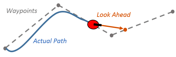
Pure pursuit
esta estrategia recibe el nombre de pure pursuit ya que se hala el punto meta para seguir empleando un control punto a punto, en lugar de usar un controlador de trayectoria
Pure pursuit
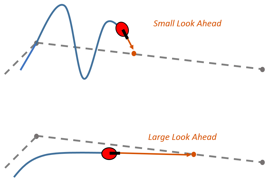
Look Ahead \(\equiv\) capacidad "predictiva"
Pure pursuit
>> mt3005_clase13_unicycle_pid.m
Términos feedforward
otra forma de dotar con capacidad predictiva al controlador PID (y el resto) es mediante términos feedforward de velocidad de control
\mathbf{v}_{ss}(t)=\mathbf{J}^\dagger\left(\boldsymbol{\xi}\right) \dot{\boldsymbol{\xi}}_d(t)
Términos feedforward
estos emplean el modelo junto con la velocidad de la trayectoria para pre-calcular la velocidad requerida por el robot en open-loop
otra forma de dotar con capacidad predictiva al controlador PID (y el resto) es mediante términos feedforward de velocidad de control
\mathbf{v}_{ss}(t)=\mathbf{J}^\dagger\left(\boldsymbol{\xi}\right) \dot{\boldsymbol{\xi}}_d(t)
Términos feedforward
feedback
(robustez)
recordemos la efectividad de la mezcla
\mathbf{v}_\mathrm{ctrl}=\mathbf{v}\left(e_p,e_o\right) \quad + \quad \mathbf{v}_{ss}(t)
feedforward
(rapidez)
\mathbf{v}\left(e_p,e_o\right)
\mathbf{v}_{ss}(t)
para "arreglar" la falta de controlabilidad puede emplearse el siguiente "truco"
(x,y)
\theta
Linealización por difeomorfismo
para "arreglar" la falta de controlabilidad puede emplearse el siguiente "truco"
(x,y)
\theta
\{
\ell_0
\left(\tilde{x}, \tilde{y}\right)
se define un nuevo punto cercano a la posición del uniciclo
\ell_0 \approx 0
Linealización por difeomorfismo
para "arreglar" la falta de controlabilidad puede emplearse el siguiente "truco"
(x,y)
\theta
\{
\ell_0
\left(\tilde{x}, \tilde{y}\right)
Linealización por difeomorfismo
idea: aproximar al uniciclo con este punto
se define un nuevo punto cercano a la posición del uniciclo
\ell_0 \approx 0
para "arreglar" la falta de controlabilidad puede emplearse el siguiente "truco"
(x,y)
\theta
\{
\ell_0
\left(\tilde{x}, \tilde{y}\right)
Linealización por difeomorfismo
idea: aproximar al uniciclo con este punto
se define un nuevo punto cercano a la posición del uniciclo
\ell_0 \approx 0
\(\Rightarrow\) necesitamos su dinámica
\tilde{x}=x+\ell_0\cos\theta \\
\tilde{y}=y+\ell_0\sin\theta
\tilde{x}=x+\ell_0\cos\theta \\
\tilde{y}=y+\ell_0\sin\theta
\dot{\tilde{x}}=\dot{x}-\ell_0\sin\theta\dot{\theta} \\
\dot{\tilde{y}}=\dot{y}+\ell_0\cos\theta\dot{\theta}
supondremos que podemos controlar | actuar directamente al punto \((\tilde{x},\tilde{y})\)
u_1
u_2
=u_1 \\
=u_2
\tilde{x}=x+\ell_0\cos\theta \\
\tilde{y}=y+\ell_0\sin\theta
\dot{\tilde{x}}=\dot{x}-\ell_0\sin\theta\dot{\theta} \\
\dot{\tilde{y}}=\dot{y}+\ell_0\cos\theta\dot{\theta}
supondremos que podemos controlar | actuar directamente al punto \((\tilde{x},\tilde{y})\)
\begin{bmatrix} \dot{\tilde{x}} \\ \dot{\tilde{y}} \end{bmatrix}=
\begin{bmatrix} \cos\theta & -\sin\theta \\ \sin\theta & \cos\theta \end{bmatrix} \begin{bmatrix} 1 & 0 \\ 0 & \ell_0 \end{bmatrix} \begin{bmatrix} v \\ \omega \end{bmatrix}
=\begin{bmatrix} u_1 \\ u_2 \end{bmatrix}
u_1
u_2
=u_1 \\
=u_2
\tilde{x}=x+\ell_0\cos\theta \\
\tilde{y}=y+\ell_0\sin\theta
\dot{\tilde{x}}=\dot{x}-\ell_0\sin\theta\dot{\theta} \\
\dot{\tilde{y}}=\dot{y}+\ell_0\cos\theta\dot{\theta}
matriz diagonal de ajuste
{^I}\mathbf{R}_B(\theta)
\begin{bmatrix} \dot{\tilde{x}} \\ \dot{\tilde{y}} \end{bmatrix}=
\begin{bmatrix} \cos\theta & -\sin\theta \\ \sin\theta & \cos\theta \end{bmatrix} \begin{bmatrix} 1 & 0 \\ 0 & \ell_0 \end{bmatrix} \begin{bmatrix} v \\ \omega \end{bmatrix}
=\begin{bmatrix} u_1 \\ u_2 \end{bmatrix}
\begin{bmatrix} v \\ \omega \end{bmatrix}=
\begin{bmatrix} 1 & 0 \\ 0 & 1/\ell_0 \end{bmatrix} {^I}\mathbf{R}_B^{-1}(\theta) \begin{bmatrix} u_1 \\ u_2 \end{bmatrix}
matriz diagonal de ajuste
{^I}\mathbf{R}_B(\theta)
\begin{bmatrix} \dot{\tilde{x}} \\ \dot{\tilde{y}} \end{bmatrix}=
\begin{bmatrix} \cos\theta & -\sin\theta \\ \sin\theta & \cos\theta \end{bmatrix} \begin{bmatrix} 1 & 0 \\ 0 & \ell_0 \end{bmatrix} \begin{bmatrix} v \\ \omega \end{bmatrix}
=\begin{bmatrix} u_1 \\ u_2 \end{bmatrix}
\mathbf{v}=
\mathbf{M}(\ell_0,\theta) \mathbf{u}
difeomorfismo que mapea las velocidades virtuales a las del uniciclo
\mathbf{M}(\ell_0,\theta)
\begin{bmatrix} v \\ \omega \end{bmatrix}=
\begin{bmatrix} 1 & 0 \\ 0 & 1/\ell_0 \end{bmatrix} {^I}\mathbf{R}_B^{-1}(\theta) \begin{bmatrix} u_1 \\ u_2 \end{bmatrix}
matriz diagonal de ajuste
{^I}\mathbf{R}_B(\theta)
\begin{bmatrix} \dot{\tilde{x}} \\ \dot{\tilde{y}} \end{bmatrix}=
\begin{bmatrix} \cos\theta & -\sin\theta \\ \sin\theta & \cos\theta \end{bmatrix} \begin{bmatrix} 1 & 0 \\ 0 & \ell_0 \end{bmatrix} \begin{bmatrix} v \\ \omega \end{bmatrix}
=\begin{bmatrix} u_1 \\ u_2 \end{bmatrix}
\begin{bmatrix} \dot{\tilde{x}} \\ \dot{\tilde{y}} \end{bmatrix}=
\begin{bmatrix} u_1 \\ u_2 \end{bmatrix}
\equiv \begin{bmatrix} \dot{\tilde{x}} \\ \dot{\tilde{y}} \end{bmatrix}=
\begin{bmatrix} 0 & 0 \\ 0 & 0 \end{bmatrix} \begin{bmatrix} \tilde{x} \\ \tilde{y} \end{bmatrix}+
\begin{bmatrix} 1 & 0 \\ 0 & 1 \end{bmatrix} \begin{bmatrix} u_1 \\ u_2 \end{bmatrix}
por lo tanto
Estabilización por LQR
\begin{bmatrix} \dot{\tilde{x}} \\ \dot{\tilde{y}} \end{bmatrix}=
\begin{bmatrix} u_1 \\ u_2 \end{bmatrix}
\equiv \begin{bmatrix} \dot{\tilde{x}} \\ \dot{\tilde{y}} \end{bmatrix}=
\begin{bmatrix} 0 & 0 \\ 0 & 0 \end{bmatrix} \begin{bmatrix} \tilde{x} \\ \tilde{y} \end{bmatrix}+
\begin{bmatrix} 1 & 0 \\ 0 & 1 \end{bmatrix} \begin{bmatrix} u_1 \\ u_2 \end{bmatrix}
por lo tanto
\dot{\mathbf{x}}
\mathbf{A}
\mathbf{x}
\mathbf{B}
\mathbf{u}
\mathbf{x}_{ss}=\begin{bmatrix} x_g \\ y_g \end{bmatrix}
\mathbf{Q}=\mathbf{R}=\mathbf{I}_2
\mathbf{v}=
\mathbf{M}(\ell_0,\theta) \mathbf{u}
Estabilización por LQR
\begin{bmatrix} \dot{\tilde{x}} \\ \dot{\tilde{y}} \end{bmatrix}=
\begin{bmatrix} u_1 \\ u_2 \end{bmatrix}
\equiv \begin{bmatrix} \dot{\tilde{x}} \\ \dot{\tilde{y}} \end{bmatrix}=
\begin{bmatrix} 0 & 0 \\ 0 & 0 \end{bmatrix} \begin{bmatrix} \tilde{x} \\ \tilde{y} \end{bmatrix}+
\begin{bmatrix} 1 & 0 \\ 0 & 1 \end{bmatrix} \begin{bmatrix} u_1 \\ u_2 \end{bmatrix}
por lo tanto
\dot{\mathbf{x}}
\mathbf{A}
\mathbf{x}
\mathbf{B}
\mathbf{u}
\mathbf{v}=
\mathbf{M}(\ell_0,\theta) \mathbf{u}
Rastreo por LQI
\mathbf{r}=\begin{bmatrix} x_g \\ y_g \end{bmatrix}
\boldsymbol{\mathcal{Q}}=\mathbf{I}_4
\boldsymbol{\mathcal{R}}=\mathbf{I}_2
\mathbf{y}_r=\begin{bmatrix} x \\ y \end{bmatrix}
\begin{bmatrix} \dot{\tilde{x}} \\ \dot{\tilde{y}} \end{bmatrix}=
\begin{bmatrix} u_1 \\ u_2 \end{bmatrix}
\equiv \begin{bmatrix} \dot{\tilde{x}} \\ \dot{\tilde{y}} \end{bmatrix}=
\begin{bmatrix} 0 & 0 \\ 0 & 0 \end{bmatrix} \begin{bmatrix} \tilde{x} \\ \tilde{y} \end{bmatrix}+
\begin{bmatrix} 1 & 0 \\ 0 & 1 \end{bmatrix} \begin{bmatrix} u_1 \\ u_2 \end{bmatrix}
por lo tanto
\dot{\mathbf{x}}
\mathbf{A}
\mathbf{x}
\mathbf{B}
\mathbf{u}
Rastreo por LQI
\mathbf{v}=
\mathbf{M}(\ell_0,\theta) \mathbf{u}
\mathbf{r}=\begin{bmatrix} x_g \\ y_g \end{bmatrix}
\boldsymbol{\mathcal{Q}}=\mathbf{I}_4
\boldsymbol{\mathcal{R}}=\mathbf{I}_2
\mathbf{y}_r=\begin{bmatrix} x \\ y \end{bmatrix}
>> mt3005_clase13_unicycle_lqrlqi.m
Regresando al robot
para el caso particular del robot diferencial podemos notar que
\dot{x}=\dfrac{r\left(\dot{\varphi}_R+\dot{\varphi}_L\right)}{2}\cos\theta
\dot{y}=\dfrac{r\left(\dot{\varphi}_R+\dot{\varphi}_L\right)}{2}\sin\theta
\dot{\theta}=\dfrac{r\left(\dot{\varphi}_R-\dot{\varphi}_L\right)}{2\ell}
\ell
\ell
r
v_r
v_\ell
Del uniciclo de regreso al robot móvil
para el caso particular del robot diferencial podemos notar que
\dot{x}=\dfrac{r\left(\dot{\varphi}_R+\dot{\varphi}_L\right)}{2}\cos\theta
\dot{y}=\dfrac{r\left(\dot{\varphi}_R+\dot{\varphi}_L\right)}{2}\sin\theta
\dot{\theta}=\dfrac{r\left(\dot{\varphi}_R-\dot{\varphi}_L\right)}{2\ell}
\ell
\ell
r
v_r
v_\ell
\(v\) del uniciclo
\(\omega\) del uniciclo
Del uniciclo de regreso al robot móvil
v=\dfrac{r\left(\dot{\varphi}_R+\dot{\varphi}_L\right)}{2}
\omega=\dfrac{r\left(\dot{\varphi}_R-\dot{\varphi}_L\right)}{2\ell}
Del uniciclo de regreso al robot móvil
para el caso particular del robot diferencial podemos notar que
v=\dfrac{r\left(\dot{\varphi}_R+\dot{\varphi}_L\right)}{2}
\omega=\dfrac{r\left(\dot{\varphi}_R-\dot{\varphi}_L\right)}{2\ell}
y entonces
\dot{\varphi}_{R,\mathrm{ctrl}}=\dfrac{v_\mathrm{ctrl}+\ell\omega_\mathrm{ctrl}}{r} \qquad
\dot{\varphi}_{L,\mathrm{ctrl}}=\dfrac{v_\mathrm{ctrl}-\ell\omega_\mathrm{ctrl}}{r}
Del uniciclo de regreso al robot móvil
para el caso particular del robot diferencial podemos notar que
La metodología para controlar robots móviles no holonómicos se resume entonces como:
- se muestra que el modelo del robot puede mapearse al uniciclo.
- se controla al uniciclo, para encontrar las velocidades de control \(v_\mathrm{ctrl}\) y \(\omega_\mathrm{ctrl}\).
- se mapean las velocidades de control de regreso al robot real.
Del uniciclo de regreso al robot móvil
Laboratorio 11
Addendum
Otros controladores para el uniciclo
Control no lineal de pose
(x,y)
\theta
(x_g,y_g)
x_B
y_B
\{G\}
x_G
y_G
\beta
\Delta x
\Delta y
\| \cdot \|_2=\rho
\{B\}
\alpha
Control no lineal de pose
Control no lineal de pose
x_B
y_B
\{G\}
x_G
y_G
\beta
\{B\}
Control no lineal de pose
(x,y)
\theta
(x_g,y_g)
x_B
y_B
\{G\}
x_G
y_G
\beta
\Delta x
\Delta y
\{B\}
Control no lineal de pose
(x,y)
\theta
(x_g,y_g)
x_B
y_B
\{G\}
x_G
y_G
\beta
\Delta x
\Delta y
\| \cdot \|_2=\rho
\{B\}
\alpha
Control no lineal de pose
(x,y)
\theta
(x_g,y_g)
x_B
y_B
\{G\}
x_G
y_G
\beta
\Delta x
\Delta y
\| \cdot \|_2=\rho
\{B\}
\alpha
se realiza el cambio de coordenadas
\rho=\sqrt{\Delta x^2 +\Delta y^2} \\
\alpha=-\theta+\mathrm{atan2}\left(\Delta y, \Delta x\right) \\
\beta=-\theta-\alpha
Control no lineal de pose
(x,y)
\theta
(x_g,y_g)
x_B
y_B
\{G\}
x_G
y_G
\beta
\Delta x
\Delta y
\| \cdot \|_2=\rho
\{B\}
\alpha
se realiza el cambio de coordenadas
\rho=\sqrt{\Delta x^2 +\Delta y^2} \\
\alpha=-\theta+\mathrm{atan2}\left(\Delta y, \Delta x\right) \\
\beta=-\theta-\alpha
OJO: esto corresponde a un mejor planteamiento del controlador PID
Control no lineal de pose
(x,y)
\theta
(x_g,y_g)
x_B
y_B
\{G\}
x_G
y_G
\beta
\Delta x
\Delta y
\| \cdot \|_2=\rho
\{B\}
\alpha
se realiza el cambio de coordenadas
\rho=\sqrt{\Delta x^2 +\Delta y^2} \\
\alpha=-\theta+\mathrm{atan2}\left(\Delta y, \Delta x\right) \\
\beta=-\theta-\alpha
puede igualmente hacerse el ajuste con
angdiffControl no lineal de pose
(x,y)
\theta
(x_g,y_g)
x_B
y_B
\{G\}
x_G
y_G
\beta
\Delta x
\Delta y
\| \cdot \|_2=\rho
\{B\}
\alpha
se realiza el cambio de coordenadas
\rho=\sqrt{\Delta x^2 +\Delta y^2} \\
\alpha=-\theta+\mathrm{atan2}\left(\Delta y, \Delta x\right) \\
\beta=-\theta-\alpha
puede igualmente hacerse el ajuste con
angdiffpuede hacerse el ajuste de acercamiento exponencial
si se restringe a \(\alpha \in \left(-\dfrac{\pi}{2},\dfrac{\pi}{2}\right) \) podemos hacer un cambio de coordenadas y obtener el nuevo sistema dinámico
\begin{bmatrix} \dot{\rho} \\ \dot{\alpha} \\ \dot{\beta} \end{bmatrix}=
\begin{bmatrix} -\cos\alpha & 0 \\ \sin\alpha/\rho & -1 \\ -\sin\alpha/\rho & 0 \end{bmatrix} \begin{bmatrix} v \\ \omega \end{bmatrix}
hace que el robot se mueva hacia adelante
puede redefinirse \(v=-v\)
\Rightarrow \begin{bmatrix} \dot{\rho} \\ \dot{\alpha} \\ \dot{\beta} \end{bmatrix}=
\begin{bmatrix} \cos\alpha & 0 \\ -\sin\alpha/\rho & 1 \\ \sin\alpha/\rho & 0 \end{bmatrix} \begin{bmatrix} v \\ \omega \end{bmatrix}
en este nuevo sistema de coordenadas, el controlador
v=k_\rho \rho \\
\omega=k_\alpha \alpha + k_\beta \beta
k_\rho>0, \quad k_\beta < 0 \\
k_\alpha+\frac{5}{3}k_\beta-\frac{2}{\pi}k_\rho>0
en este nuevo sistema de coordenadas, el controlador
v=k_\rho \rho \\
\omega=k_\alpha \alpha + k_\beta \beta
k_\rho>0, \quad k_\beta < 0 \\
k_\alpha+\frac{5}{3}k_\beta-\frac{2}{\pi}k_\rho>0
garantiza que el punto \((\rho,\alpha,\beta)=(0,0,0)\) sea globalmente asintóticamente estable...
en este nuevo sistema de coordenadas, el controlador
v=k_\rho \rho \\
\omega=k_\alpha \alpha + k_\beta \beta
k_\rho>0, \quad k_\beta < 0 \\
k_\alpha+\frac{5}{3}k_\beta-\frac{2}{\pi}k_\rho>0
garantiza que el punto \((\rho,\alpha,\beta)=(0,0,0)\) sea globalmente asintóticamente estable...
... y que no cambie de dirección de movimiento al acercarse a la meta
en este nuevo sistema de coordenadas, el controlador
v=k_\rho \rho \\
\omega=k_\alpha \alpha + k_\beta \beta
k_\rho>0, \quad k_\beta < 0 \\
k_\alpha+\frac{5}{3}k_\beta-\frac{2}{\pi}k_\rho>0
garantiza que el punto \((\rho,\alpha,\beta)=(0,0,0)\) sea globalmente asintóticamente estable...
>> mt3005_clase13_unicycle_nonlin.m
en este nuevo sistema de coordenadas, el controlador
v=k_\rho \rho \\
\omega=k_\alpha \alpha + k_\beta \beta
k_\rho>0, \quad k_\beta < 0 \\
k_\alpha+\frac{5}{3}k_\beta-\frac{2}{\pi}k_\rho>0
garantiza que el punto \((\rho,\alpha,\beta)=(0,0,0)\) sea globalmente asintóticamente estable...
NOTA: este controlador siempre "parquea" al robot con su eje \(x\) alineado con el del marco \(\{G\}\).
k_\rho>0, \quad k_\beta < 0 \\
k_\alpha+\frac{5}{3}k_\beta-\frac{2}{\pi}k_\rho>0
en este nuevo sistema de coordenadas, el controlador
v=k_\rho \rho \\
\omega=k_\alpha \alpha + k_\beta \beta
garantiza que el punto \((\rho,\alpha,\beta)=(0,0,0)\) sea globalmente asintóticamente estable...
NOTA: este controlador siempre "parquea" al robot con su eje \(x\) alineado con el del marco \(\{G\}\).
OJO: existen muchos más controladores para el uniciclo, sin embargo los anteriores muestrean un poco de todo lo que hemos visto en los cursos de Sistemas de Control
MT3005 - Lecture 13 (2025)
By Miguel Enrique Zea Arenales


