Introducción al filtro de Kalman
IE3041 - Sistemas de Control 2

La forma correcta de utilizar el "LQR" para observadores
Del LQR al filtro de Kalman
recordemos que la idea del LQR fue penalizar divergencia en las variables de estado y un sobre-uso de los actuadores (entradas)
Del LQR al filtro de Kalman
recordemos que la idea del LQR fue penalizar divergencia en las variables de estado y un sobre-uso de los actuadores (entradas)
\begin{aligned}
\mathbf{u}^\star(t) = & \displaystyle\arg\min_{\mathbf{u}(t)} \displaystyle\int_{t_0}^{\infty} \left[\mathbf{x}(t)^\top \mathbf{Q}\mathbf{x}(t)+\mathbf{u}(t)^\top \mathbf{R}\mathbf{u}(t)\right]dt \\
& \textrm{s.t.} \quad \dot{\mathbf{x}}=\mathbf{A}\mathbf{x}+\mathbf{B}\mathbf{u} \\
\end{aligned}
Del LQR al filtro de Kalman
¿Qué ocurre si quisiéramos modificarlo para emplear la dinámica del observador de Luenberger?
\begin{aligned}
\mathbf{u}^\star(t) = & \displaystyle\arg\min_{\mathbf{u}(t)} \displaystyle\int_{t_0}^{\infty} \left[\mathbf{x}(t)^\top \mathbf{Q}\mathbf{x}(t)+\mathbf{u}(t)^\top \mathbf{R}\mathbf{u}(t)\right]dt \\
& \textrm{s.t.} \quad \dot{\mathbf{x}}=\mathbf{A}\mathbf{x}+\mathbf{B}\mathbf{u} \\
\end{aligned}
\dot{\mathbf{e}}=\left(\mathbf{A}-\mathbf{L}\mathbf{C}\right)\mathbf{e}
\ \mathbf{e}(t)
\ \mathbf{e}(t)
+ \ \square
???
Resulta que no sólo la entrada es fundamental para el planteamiento del LQR sino que este deja de existir al no estar presente esta
Del LQR al filtro de Kalman
entonces, para que el "LQR de observadores" funcione, debe penalizar algo en el lugar de la entrada
Del LQR al filtro de Kalman
entonces, para que el "LQR de observadores" funcione, debe penalizar algo en el lugar de la entrada
resulta que la respuesta a esto corresponde al ruido en el sistema
Del LQR al filtro de Kalman
entonces, para que el "LQR de observadores" funcione, debe penalizar algo en el lugar de la entrada
resulta que la respuesta a esto corresponde al ruido en el sistema
sin embargo, para entender el planteamiento necesitamos ser capaces de describir señales aleatorias
Del LQR al filtro de Kalman
entonces, para que el "LQR de observadores" funcione, debe penalizar algo en el lugar de la entrada
resulta que la respuesta a esto corresponde al ruido en el sistema
sin embargo, para entender el planteamiento necesitamos ser capaces de describir señales aleatorias
pongamos esto en contexto con un ejemplo...
Sensores
\ t
x(t)
\ t
x(t)
señal + ruido
\ t
x(t)
señal + ruido
PROBLEMA
aún tenemos pendiente desarrollar herramientas matemáticas para lidiar con el ruido
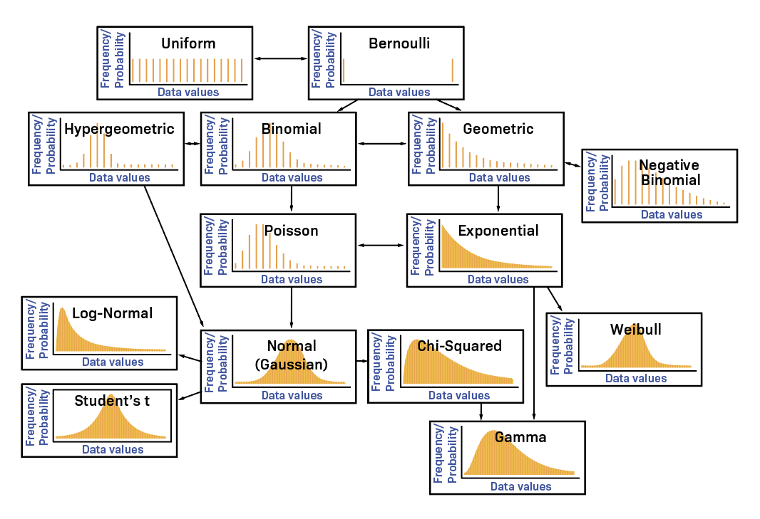
Probabilidad y variables aleatorias
x = -2.35893
x = -2.35893
X =
posibles valores
x = -2.35893
X =
posibles valores
existe cierta probabilidad que tome algún valor en específico dentro de los posibles
x = -2.35893
X =
posibles valores
\(\Rightarrow X\) es una variable aleatoria
existe cierta probabilidad que tome algún valor en específico dentro de los posibles
descrita por una función de densidad probabilística (pdf)
existe cierta probabilidad que tome algún valor en específico dentro de los posibles
descrita por una función de densidad probabilística (pdf)
\(P(X=x)=f_X(x)\) tal que \(\displaystyle\int_{-\infty}^{\infty}f_X(x)dx=1\)
existe cierta probabilidad que tome algún valor en específico dentro de los posibles
Ejemplo: variable aleatoria discreta

1
1/6
\ x
f_X(x)
2
3
4
5
6
Ejemplo: variable aleatoria discreta
P(X=2)=f_X(2)=1/6
P(X>3)=\displaystyle\int_{3}^{\infty}f_X(x)dx=1/2
1
1/6
\ x
f_X(x)
2
3
4
5
6
Ejemplo: variable aleatoria discreta
X \sim \mathcal{U}\{1,6\}
distribución uniforme discreta
1
1/6
\ x
f_X(x)
2
3
4
5
6
P(X=2)=f_X(2)=1/6
P(X>3)=\displaystyle\int_{3}^{\infty}f_X(x)dx=1/2
Ejemplo: distribución uniforme continua
a
b
\dfrac{1}{b-a}
\ x
f_X(x)
X \sim \mathcal{U}(a,b)
Ejemplo: distribución uniforme continua
a
b
\dfrac{1}{b-a}
\ x
f_X(x)
X \sim \mathcal{U}(a,b)
P(X=2)=\mathrm{cte.}
P(X=4.75)=\mathrm{cte.}
a
b
\dfrac{1}{b-a}
\ x
X \sim \mathcal{U}(a,b)
P(X=2)=\mathrm{cte.}
P(X=4.75)=\mathrm{cte.}
X \sim \mathcal{U}(2,8)
=2
=8
=\dfrac{1}{6}
Ejemplo: distribución uniforme continua
f_X(x)
Ejemplo: distribución normal (Gaussiana)
\ x
f_X(x)
X \sim \mathcal{N}\left(\mu,\sigma^2\right)
Ejemplo: distribución normal (Gaussiana)
\ x
f_X(x)
X \sim \mathcal{N}\left(\mu,\sigma^2\right)
\mu
media o promedio
Ejemplo: distribución normal (Gaussiana)
\ x
f_X(x)
X \sim \mathcal{N}\left(\mu,\sigma^2\right)
\mu
media o promedio
\sigma^2
varianza o el cuadrado de la desviación estándar
Ejemplo: distribución normal (Gaussiana)
\ x
f_X(x)
\mu
media o promedio
\sigma^2
varianza o el cuadrado de la desviación estándar
f_X(x)=\dfrac{1}{\sigma\sqrt{2\pi}}e^{-\frac{1}{2}\left(\frac{x-\mu}{\sigma}\right)^2}
Ejemplo: distribución normal (Gaussiana)
\ x
f_X(x)
X \sim \mathcal{N}\left(0,1\right)
distribución normal estándar
-1
1
0
Ejemplo: distribución normal (Gaussiana)
\ x
-1
1
0
a veces se busca pero la probabilidad acumulada hasta cierto valor
P(X\le -1)=F_X(-1)
f_X(x)
X \sim \mathcal{N}\left(0,1\right)
distribución normal estándar
Ejemplo: distribución normal (Gaussiana)
\ x
-1
1
0
a veces se busca pero la probabilidad acumulada hasta cierto valor
P(X\le -1)=F_X(-1)
F_X(x)=\displaystyle\int_{-\infty}^{x}f_X(s)ds
cdf
f_X(x)
X \sim \mathcal{N}\left(0,1\right)
distribución normal estándar
Otras distribuciones
Múltiples variables aleatorias
supongamos que ahora se tienen dos variables aleatorias \(X\) y \(Y\), entonces, se define su distribución de probabilidad conjunta (joint pdf) como
P(X=x, Y=y)=f_{XY}(x,y)
P(X=x, Y=y)=f_{XY}(x,y)
sí y sólo si \(X\) y \(Y\) son independientes
f_{XY}(x,y)=f_X(x)f_Y(y)
supongamos que ahora se tienen dos variables aleatorias \(X\) y \(Y\), entonces, se define su distribución de probabilidad conjunta (joint pdf) como
Múltiples variables aleatorias
Medidas, momentos y valor esperado
la media y la varianza describen a las distribuciones normales, sin embargo, resulta que forman parte de un conjunto de medidas que aplica a cualquier tipo de distribución
Medidas, momentos y valor esperado
la media y la varianza describen a las distribuciones normales, sin embargo, resulta que forman parte de un conjunto de medidas que aplica a cualquier tipo de distribución
la mayoría requiere de la noción general de valor esperado para calcularse
E_X[x]=\displaystyle\int_{-\infty}^{\infty}xf_X(x)dx
valor esperado (promedio ponderado)
E_X[x]=\displaystyle\int_{-\infty}^{\infty}xf_X(x)dx
\mu_X=E_X[x]
\sigma_X^2=E_X\left[(x-\mu_X)^2\right]
\rho_{XY}=\dfrac{\sigma_{XY}}{\sigma_X\sigma_Y}
\sigma_{XY}=E_{XY}\left[(x-\mu_X)(y-\mu_Y)\right]
valor esperado (promedio ponderado)
covarianza
correlación
varianza
media
Otras medidas
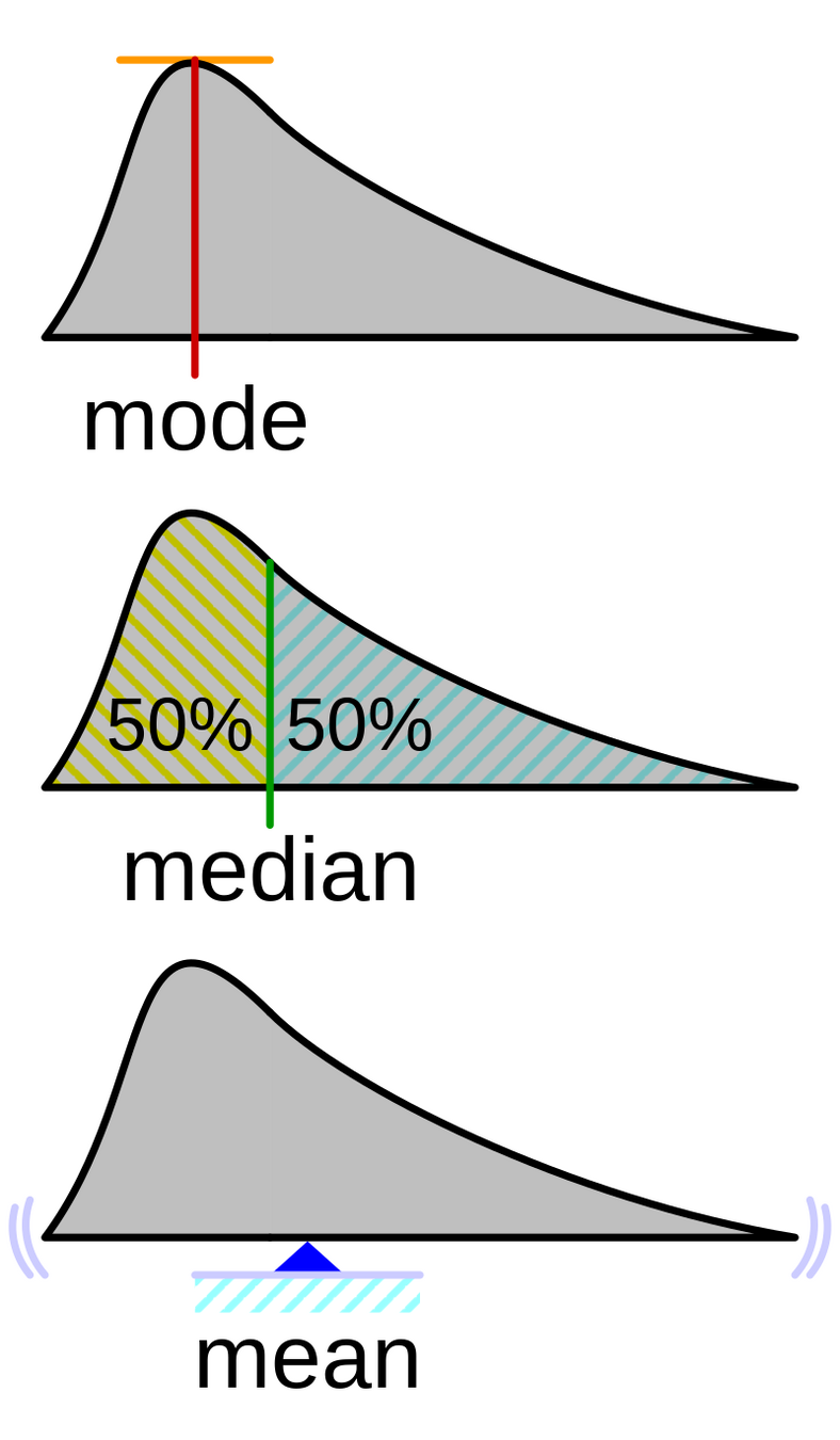
\mathrm{mode}=\argmax_x f_X(x)
\lim_{x \to m^-} F_X(x) \le \dfrac{1}{2} \le F_X(m)
(m)
estas reciben el nombre de medidas de tendencia central
Varianza vs covarianza
>> ie3041_clase9_gaussianas.m
mientras la varianza es una medida de dispersión, la covarianza (y correlación) es una medida que representa la relación lineal entre las variables aleatorias, es decir, en qué medida el cambio de una está relacionado con el de la otra
Vectores de variables aleatorias
para evitar la confusión con matrices, emplearemos una notación distinta para vectores de variables aleatorias, por ejemplo, para el caso con \(\mathbf{x}\in\mathbb{R}^n\)
\boldsymbol{\mu}_\mathbf{x}=E\left\{\mathbf{x}\right\}=E\left\{\begin{bmatrix} x_1 \\ x_2 \\ \vdots \\ x_n \end{bmatrix}\right\}
=\begin{bmatrix} E\{x_1\} \\ E\{x_2\} \\ \vdots \\ E\{x_n\} \end{bmatrix}
adicionalmente, las varianzas y covarianzas se combinan en un único objeto denominado matriz de covarianza
\mathbf{Q}_\mathbf{x}=\mathbf{Q}^\top_\mathbf{x}=E\left\{(\mathbf{x}-\mu_\mathbf{x})(\mathbf{x}-\mu_\mathbf{x})^\top\right\}
Vectores de variables aleatorias
adicionalmente, las varianzas y covarianzas se combinan en un único objeto denominado matriz de covarianza
\mathbf{Q}_\mathbf{x}=\mathbf{Q}^\top_\mathbf{x}=E\left\{(\mathbf{x}-\mu_\mathbf{x})(\mathbf{x}-\mu_\mathbf{x})^\top\right\}
varianzas en la diagonal y covarianzas fuera de la diagonal
Vectores de variables aleatorias
Ejemplo: Gaussiana de 3 dimensiones
\mathbf{x}=\begin{bmatrix} x_1 \\ x_2 \\ x_3 \end{bmatrix} \begin{matrix} \sim \mathcal{N}(0,1) \\ \sim \mathcal{N}(0,1) \\ \sim \mathcal{N}(0,1) \end{matrix}
Ejemplo: Gaussiana de 3 dimensiones
\mathbf{x}=\begin{bmatrix} x_1 \\ x_2 \\ x_3 \end{bmatrix} \begin{matrix} \sim \mathcal{N}(0,1) \\ \sim \mathcal{N}(0,1) \\ \sim \mathcal{N}(0,1) \end{matrix}
\Rightarrow \mathbf{x}\sim\mathcal{N}\left(\mathbf{0}, \mathbf{Q}_\mathbf{x}\right)
Ejemplo: Gaussiana de 3 dimensiones
\mathbf{x}=\begin{bmatrix} x_1 \\ x_2 \\ x_3 \end{bmatrix} \begin{matrix} \sim \mathcal{N}(0,1) \\ \sim \mathcal{N}(0,1) \\ \sim \mathcal{N}(0,1) \end{matrix}
\Rightarrow \mathbf{x}\sim\mathcal{N}\left(\mathbf{0}, \mathbf{Q}_\mathbf{x}\right)
f(\mathbf{x})=\dfrac{1}{\sqrt{(2\pi)^n\det(\mathbf{Q}_\mathbf{x})}}e^{-\frac{1}{2}(\mathbf{x}-\boldsymbol{\mu})^\top\mathbf{Q}_\mathbf{x}^{-1}(\mathbf{x}-\boldsymbol{\mu})}
\mathbf{Q}_\mathbf{x}=E\left\{(\mathbf{x}-\mathbf{0})(\mathbf{x}-\mathbf{0})^\top\right\}=E\left\{\mathbf{x}\mathbf{x}^\top\right\}
Ejemplo: Gaussiana de 3 dimensiones
\mathbf{Q}_\mathbf{x}=E\left\{(\mathbf{x}-\mathbf{0})(\mathbf{x}-\mathbf{0})^\top\right\}=E\left\{\mathbf{x}\mathbf{x}^\top\right\}
\mathbf{Q}_\mathbf{x}=E\left\{ \begin{bmatrix} x_1^2 & x_1x_2 & x_1x_3 \\ x_2x_1 & x_2^2 & x_2x_3 \\ x_3x_1 & x_3x_2 & x_3^2 \end{bmatrix} \right\}
Ejemplo: Gaussiana de 3 dimensiones
\mathbf{Q}_\mathbf{x}=E\left\{(\mathbf{x}-\mathbf{0})(\mathbf{x}-\mathbf{0})^\top\right\}=E\left\{\mathbf{x}\mathbf{x}^\top\right\}
\mathbf{Q}_\mathbf{x}=\begin{bmatrix} E\{x_1^2\} & E\{x_1x_2\} & E\{x_1x_3\} \\
E\{x_2x_1\} & E\{x_2^2\} & E\{x_2x_3\} \\
E\{x_3x_1\} & E\{x_3x_2\} & E\{x_3^2\} \end{bmatrix}
Ejemplo: Gaussiana de 3 dimensiones
\mathbf{Q}_\mathbf{x}=E\left\{(\mathbf{x}-\mathbf{0})(\mathbf{x}-\mathbf{0})^\top\right\}=E\left\{\mathbf{x}\mathbf{x}^\top\right\}
\mathbf{Q}_\mathbf{x}=\begin{bmatrix} \sigma_{x_1}^2 & \sigma_{x_1x_2} & \sigma_{x_1x_3} \\
\sigma_{x_1x_2} & \sigma_{x_2}^2 & \sigma_{x_2x_3} \\
\sigma_{x_1x_3} & \sigma_{x_2x_3} & \sigma_{x_3}^2 \end{bmatrix}
varianzas y el resto son covarianzas
Ejemplo: Gaussiana de 3 dimensiones
Procesos estocásticos
proceso estocástico \(x(t)\) \(\approx\) generador de variables aleatorias en el tiempo
x(t_1)\sim \mathcal{N}(0, \sigma^2)
proceso estocástico \(x(t)\) \(\approx\) generador de variables aleatorias en el tiempo
x(t_1)\sim \mathcal{N}(0, \sigma^2)
x(t_2)\sim \mathcal{U}(0, 1)
proceso estocástico \(x(t)\) \(\approx\) generador de variables aleatorias en el tiempo
x(t_1)\sim \mathcal{N}(0, \sigma^2)
x(t_2)\sim \mathcal{U}(0, 1)
x(t_3)\sim \mathcal{N}(10, 2\sigma^2)
proceso estocástico \(x(t)\) \(\approx\) generador de variables aleatorias en el tiempo
x(t_1)\sim \mathcal{N}(0, \sigma^2)
x(t_2)\sim \mathcal{U}(0, 1)
x(t_3)\sim \mathcal{N}(10, 2\sigma^2)
x(t_4)\sim \chi^2(k)
\cdots
proceso estocástico \(x(t)\) \(\approx\) generador de variables aleatorias en el tiempo
proceso estocástico \(x(t)\) \(\approx\) generador de variables aleatorias en el tiempo
x(t_1)\sim \mathcal{N}(0, \sigma^2)
x(t_2)\sim \mathcal{U}(0, 1)
x(t_3)\sim \mathcal{N}(10, 2\sigma^2)
x(t_4)\sim \chi^2(k)
\cdots
demasiado complicado, quisiéramos que las variables salgan del mismo tipo de distribución con por lo menos la misma media
E\left\{x(t_1)\right\}=E\left\{x(t_2)\right\}=\cdots
antes de simplificar necesitamos definir
r_{xx}(t_1,t_2)=E\left\{x(t_1)x(t_2)\right\}
auto-correlación
antes de simplificar necesitamos definir
r_{xx}(t_1,t_2)=E\left\{x(t_1)x(t_2)\right\}
k_{xx}(t_1,t_2)=E\left\{(x(t_1)-\mu_{t_1})(x(t_2)-\mu_{t_2})\right\}
auto-correlación
auto-covarianza
Procesos WSS
un proceso estocástico es (weak o) wide-sense stationary si cumple con
Procesos WSS
un proceso estocástico es (weak o) wide-sense stationary si cumple con
E\left\{x(t_1)\right\}=E\left\{x(t_2)\right\}=\cdots=\mu_x
Procesos WSS
un proceso estocástico es (weak o) wide-sense stationary si cumple con
E\left\{x(t_1)\right\}=E\left\{x(t_2)\right\}=\cdots=\mu_x
k_{xx}(t_1,t_2)=k_{xx}(t, t+\tau) \triangleq k_{xx}(\tau)
Procesos WSS
un proceso estocástico es (weak o) wide-sense stationary si cumple con
E\left\{x(t_1)\right\}=E\left\{x(t_2)\right\}=\cdots=\mu_x
r_{xx}(t_1,t_2)=r_{xx}(t, t+\tau) \triangleq r_{xx}(\tau)
Procesos WSS
un proceso estocástico es (weak o) wide-sense stationary si cumple con
E\left\{x(t_1)\right\}=E\left\{x(t_2)\right\}=\cdots=\mu_x
r_{xx}(t_1,t_2)=r_{xx}(t, t+\tau) \triangleq r_{xx}(\tau)
E\left\{|x(t)|^2\right\} < \infty
Procesos WSS
un proceso estocástico es (weak o) wide-sense stationary si cumple con
E\left\{x(t_1)\right\}=E\left\{x(t_2)\right\}=\cdots=\mu_x
r_{xx}(t_1,t_2)=r_{xx}(t, t+\tau) \triangleq r_{xx}(\tau)
E\left\{|x(t)|^2\right\} < \infty
Nota: el procesamiento de señales estocásticas usa la auto-correlación como la señal de tiempo y aplica (casi) los mismos métodos. Por ejemplo:
R_{xx}(\jmath\Omega)=\mathcal{F}\left\{r_{xx}(\tau)\right\}
Power Spectral Density (PSD)
Ejemplo: ruido blanco
ruido Gaussiano no correlacionado
Ejemplo: ruido blanco
ruido Gaussiano no correlacionado
r_{xx}(\tau)=\sigma^2\delta(\tau)
\ \tau
Ejemplo: ruido blanco
ruido Gaussiano no correlacionado
\ \tau
conocer algo del proceso en el tiempo \(t_1\) no nos dice nada sobre el proceso en el tiempo \(t_2\)
>> ie3041_clase9_ruidoblanco.m
r_{xx}(\tau)=\sigma^2\delta(\tau)
Regresando al filtro de Kalman
INTENSE
dado que queremos una herramienta lineal que podamos aplicar a sistemas no lineales, es necesario emplear el planteamiento "original" (completo) del filtro
dado que queremos una herramienta lineal que podamos aplicar a sistemas no lineales, es necesario emplear el planteamiento "original" (completo) del filtro
este asume un sistema LTV estocástico
Un ajuste al modelo lineal

Un ajuste al modelo lineal
\dot{\mathbf{x}}=\mathbf{A}(t)\mathbf{x}+\mathbf{B}(t)\mathbf{u}+\mathbf{F}(t)\mathbf{w} \\
\mathbf{y}=\mathbf{C}(t)\mathbf{x}+\mathbf{v}
Un ajuste al modelo lineal
ruido de proceso
vector de ruido blanco
ruido de medición
vector de ruido blanco
\dot{\mathbf{x}}=\mathbf{A}(t)\mathbf{x}+\mathbf{B}(t)\mathbf{u}+\mathbf{F}(t)\mathbf{w} \\
\mathbf{y}=\mathbf{C}(t)\mathbf{x}+\mathbf{v}
Un ajuste al modelo lineal
\dot{\mathbf{x}}=\mathbf{A}(t)\mathbf{x}+\mathbf{B}(t)\mathbf{u}+\mathbf{F}(t)\mathbf{w} \\
\mathbf{y}=\mathbf{C}(t)\mathbf{x}+\mathbf{v}
\mathbf{w}(t) \sim \mathcal{N}\left(\mathbf{0}, \mathbf{Q}_\mathbf{w}(t)\right)
\mathbf{v}(t) \sim \mathcal{N}\left(\mathbf{0}, \mathbf{Q}_\mathbf{v}(t)\right)
aunque se permite que cambie la varianza en el tiempo, no es lo típico
Un ajuste al modelo lineal
\dot{\mathbf{x}}=\mathbf{A}(t)\mathbf{x}+\mathbf{B}(t)\mathbf{u}+\mathbf{F}(t)\mathbf{w} \\
\mathbf{y}=\mathbf{C}(t)\mathbf{x}+\mathbf{v}
\mathbf{R}_\mathbf{w}(\tau)= E\left\{ \mathbf{w}(t) \mathbf{w}(t+\tau)^\top \right\}=\mathbf{Q}_\mathbf{w}\delta(\tau)
\mathbf{R}_\mathbf{v}(\tau)= E\left\{ \mathbf{v}(t) \mathbf{v}(t+\tau)^\top \right\}=\mathbf{Q}_\mathbf{v}\delta(\tau)
E\left\{ \mathbf{w}(t) \mathbf{v}(t)^\top \right\}=\mathbf{0}
bajo esto ya hace sentido plantear un "LQR" para observadores
\dot{\hat{\mathbf{x}}}=\mathbf{A}(t)\hat{\mathbf{x}}+\mathbf{B}(t)\mathbf{u}+\mathbf{L}(t)\left(\mathbf{y}-\hat{\mathbf{y}}\right)
\dot{\hat{\mathbf{x}}}=\mathbf{A}(t)\hat{\mathbf{x}}+\mathbf{B}(t)\mathbf{u}+\mathbf{L}(t)\left(\mathbf{y}-\hat{\mathbf{y}}\right)
\mathbf{e}=\mathbf{x}-\hat{\mathbf{x}}
\Rightarrow \dot{\mathbf{e}}=\dot{\mathbf{x}}-\dot{\hat{\mathbf{x}}}=
\cdots
\dot{\hat{\mathbf{x}}}=\mathbf{A}(t)\hat{\mathbf{x}}+\mathbf{B}(t)\mathbf{u}+\mathbf{L}(t)\left(\mathbf{y}-\hat{\mathbf{y}}\right)
\mathbf{e}=\mathbf{x}-\hat{\mathbf{x}}
\Rightarrow \dot{\mathbf{e}}=\dot{\mathbf{x}}-\dot{\hat{\mathbf{x}}}=
\cdots
\dot{\mathbf{e}}=\left(\mathbf{A}(t)-\mathbf{L}(t)\mathbf{C}(t)\right)\mathbf{e}+\mathbf{F}(t)\mathbf{w}-\mathbf{L(t)}\mathbf{v}
\dot{\hat{\mathbf{x}}}=\mathbf{A}(t)\hat{\mathbf{x}}+\mathbf{B}(t)\mathbf{u}+\mathbf{L}(t)\left(\mathbf{y}-\hat{\mathbf{y}}\right)
\dot{\mathbf{e}}=\left(\mathbf{A}(t)-\mathbf{L}(t)\mathbf{C}(t)\right)\mathbf{e}+\mathbf{F}(t)\mathbf{w}-\mathbf{L(t)}\mathbf{v}
ya tenemos qué penalizar en lugar de la entrada \(\to\) ruido
\mathbf{e}=\mathbf{x}-\hat{\mathbf{x}}
\Rightarrow \dot{\mathbf{e}}=\dot{\mathbf{x}}-\dot{\hat{\mathbf{x}}}=
\cdots
y entonces
\mathbf{L}^\star(t)=\mathbf{P}(t)\mathbf{C}^\top(t)\mathbf{Q}_\mathbf{v}^{-1}
y entonces
\mathbf{L}^\star(t)=\mathbf{P}(t)\mathbf{C}^\top(t)\mathbf{Q}_\mathbf{v}^{-1}
ganancia de Kalman
y entonces
\mathbf{L}^\star(t)=\mathbf{P}(t)\mathbf{C}^\top(t)\mathbf{Q}_\mathbf{v}^{-1}
en donde \(\mathbf{P}=\mathbf{P}^\top \succ 0\) es la matriz de covarianza del error de estimación...
\mathbf{P}(t)=E\left\{ \left(\mathbf{x}-\hat{\mathbf{x}}\right) \left(\mathbf{x}-\hat{\mathbf{x}}\right)^\top \right\}
ganancia de Kalman
... y cuya dinámica satisface la ecuación (diferencial) de Riccati, ...
\dot{\mathbf{P}}(t)=\mathbf{A}(t)\mathbf{P}(t)+\mathbf{P}(t)\mathbf{A}^\top(t) \\
-\mathbf{P}(t)\mathbf{C}^\top(t)\mathbf{Q}_\mathbf{v}^{-1}\mathbf{C}(t)\mathbf{P}(t)
+\mathbf{F}(t)\mathbf{Q}_\mathbf{w}(t)\mathbf{F}^\top(t)
... y cuya dinámica satisface la ecuación (diferencial) de Riccati, ...
\dot{\mathbf{P}}(t)=\mathbf{A}(t)\mathbf{P}(t)+\mathbf{P}(t)\mathbf{A}^\top(t) \\
-\mathbf{P}(t)\mathbf{C}^\top(t)\mathbf{Q}_\mathbf{v}^{-1}\mathbf{C}(t)\mathbf{P}(t)
+\mathbf{F}(t)\mathbf{Q}_\mathbf{w}(t)\mathbf{F}^\top(t)
... con condiciones iniciales
\mathbf{P}(0)=E\left\{\mathbf{x}_0\mathbf{x}_0^\top\right\} \triangleq \sigma_e^2 \mathbf{I}
... con condiciones iniciales
\mathbf{P}(0)=E\left\{\mathbf{x}_0\mathbf{x}_0^\top\right\} \triangleq \sigma_e^2 \mathbf{I}
\(\mathbf{P}(0)\) representa la covarianza de la condición inicial y \(\sigma_e^2\) se utiliza para representar qué tan seguros estamos de conocerla
... con condiciones iniciales
\mathbf{P}(0)=E\left\{\mathbf{x}_0\mathbf{x}_0^\top\right\} \triangleq \sigma_e^2 \mathbf{I}
\(\mathbf{P}(0)\) representa la covarianza de la condición inicial y \(\sigma_e^2\) se utiliza para representar qué tan seguros estamos de conocerla
en conclusión, lo que busca el filtro de Kalman es minimizar \(\mathbf{P}(t)\)
>> ie3041_clase9_ctkalman.m
Un caso especial
si el sistema es LTI y las covarianzas no cambian en el tiempo, entonces
\mathbf{L}^\star=\mathbf{P}\mathbf{C}^\top\mathbf{Q}_\mathbf{v}^{-1}
si el sistema es LTI y las covarianzas no cambian en el tiempo, entonces
y \(\mathbf{P}\) ya sólo debe cumplir con la ecuación algebraica de Riccati
\mathbf{L}^\star=\mathbf{P}\mathbf{C}^\top\mathbf{Q}_\mathbf{v}^{-1}
\mathbf{0}=\mathbf{A}\mathbf{P}+\mathbf{P}\mathbf{A}^\top
-\mathbf{P}\mathbf{C}^\top\mathbf{Q}_\mathbf{v}^{-1}\mathbf{C}\mathbf{P}
+\mathbf{F}\mathbf{Q}_\mathbf{w}\mathbf{F}^\top
este recibe el nombre de filtro de Kalman en estado estacionario y corresponde al "equivalente" al LQR pero para observadores de estado
este recibe el nombre de filtro de Kalman en estado estacionario y corresponde al "equivalente" al LQR pero para observadores de estado
L = lqe(A, F, C, Qw, Qv)este recibe el nombre de filtro de Kalman en estado estacionario y corresponde al "equivalente" al LQR pero para observadores de estado
L = lqe(A, F, C, Qw, Qv)>> ie3041_clase9_lqgcontrol.m
Regresando a sistemas no lineales
\dot{\mathbf{x}}=\mathbf{f}\left(\mathbf{x},\mathbf{u},\mathbf{w}\right) \\
\mathbf{y}=\mathbf{h}\left(\mathbf{x}\right)+\mathbf{v}
si el modelo ahora cambia a uno no lineal
(y se mantienen las mismas cantidades estocásticas que se definieron anteriormente)
la dinámica para el estimador cambia a
\dot{\hat{\mathbf{x}}}=\mathbf{f}\left(\hat{\mathbf{x}},\mathbf{u},\mathbf{0}\right)+\mathbf{L}(t)\left(\mathbf{y}-\mathbf{h}\left(\hat{\mathbf{x}}\right)\right)
la dinámica para el estimador cambia a
\dot{\hat{\mathbf{x}}}=\mathbf{f}\left(\hat{\mathbf{x}},\mathbf{u},\mathbf{0}\right)+\mathbf{L}(t)\left(\mathbf{y}-\mathbf{h}\left(\hat{\mathbf{x}}\right)\right)
pero mantiene la misma ganancia de Kalman y cumple con la misma ecuación diferencial de Riccati, pero empleando matrices obtenidas mediante linealización
\mathbf{A}(t)=\dfrac{\partial \mathbf{f}\left(\hat{\mathbf{x}}, \mathbf{u}, \mathbf{0}\right)}{\partial \mathbf{x}}
\mathbf{B}(t)=\dfrac{\partial \mathbf{f}\left(\hat{\mathbf{x}}, \mathbf{u}, \mathbf{0}\right)}{\partial \mathbf{u}}
\mathbf{F}(t)=\dfrac{\partial \mathbf{f}\left(\hat{\mathbf{x}}, \mathbf{u}, \mathbf{0}\right)}{\partial \mathbf{w}}
\mathbf{C}(t)=\dfrac{\partial \mathbf{h}\left(\hat{\mathbf{x}}\right)}{\partial \mathbf{x}}
este estimador recibe el nombre de filtro de Kalman Extendido (EKF)
\mathbf{A}(t)=\dfrac{\partial \mathbf{f}\left(\hat{\mathbf{x}}, \mathbf{u}, \mathbf{0}\right)}{\partial \mathbf{x}}
\mathbf{B}(t)=\dfrac{\partial \mathbf{f}\left(\hat{\mathbf{x}}, \mathbf{u}, \mathbf{0}\right)}{\partial \mathbf{u}}
\mathbf{F}(t)=\dfrac{\partial \mathbf{f}\left(\hat{\mathbf{x}}, \mathbf{u}, \mathbf{0}\right)}{\partial \mathbf{w}}
\mathbf{C}(t)=\dfrac{\partial \mathbf{h}\left(\hat{\mathbf{x}}\right)}{\partial \mathbf{x}}
El filtro de Kalman Extendido
si bien el EKF funciona*, ya no es óptimo para el sistema no lineal y se vuelve más sensible a la correcta estimación de las condiciones iniciales
El filtro de Kalman Extendido
si bien el EKF funciona*, ya no es óptimo para el sistema no lineal y se vuelve más sensible a la correcta estimación de las condiciones iniciales
existen otras variantes del filtro que evitan el proceso de linealización, como el Unscented Kalman Filter (UKF)
IMPORTANTE
el planteamiento de tiempo continuo que vimos para tanto el filtro de Kalman como el EKF no es el que típicamente se emplea para su implementación
(sin embargo, para este curso, no nos preocuparemos al respecto de esto)
IMPORTANTE
LQR + Kalman
= Linear-Quadratic-Gaussian Control (LQG)
IMPORTANTE
LQR + Kalman
= Linear-Quadratic-Gaussian Control (LQG)
OJO: este pierde la robustez del LQR, es decir, no pueden darse garantías con respecto a sus márgenes de estabilidad
IMPORTANTE
LQR + Kalman
= Linear-Quadratic-Gaussian Control (LQG)
OJO: este pierde la robustez del LQR, es decir, no pueden darse garantías con respecto a sus márgenes de estabilidad
>> ie3041_clase9_lqgcontrol.m
IE3041 - Lecture 9 (2025)
By Miguel Enrique Zea Arenales


