Estabilización de sistemas no lineales mediante linealización
IE3041 - Sistemas de Control 2

Regresando a sistemas no lineales
similar al caso de estabilidad, tratemos de aplicar las herramientas de estabilización desarrolladas para sistemas LTI pero en el caso de sistemas no lineales
\dot{\mathbf{x}}=\mathbf{f}\left(\mathbf{x},\mathbf{u}\right) \\
\mathbf{y}=\mathbf{h}\left(\mathbf{x},\mathbf{u}\right)
\dot{\mathbf{x}}=\mathbf{f}\left(\mathbf{x},\mathbf{u}\right) \\
\mathbf{y}=\mathbf{h}\left(\mathbf{x},\mathbf{u}\right)
\left(\mathbf{x}^*,\mathbf{u}^*\right) \text{ o }\\
\left(\mathbf{x}_{ss},\mathbf{u}_{ss}\right)
\dot{\mathbf{x}}=\mathbf{f}\left(\mathbf{x},\mathbf{u}\right) \\
\mathbf{y}=\mathbf{h}\left(\mathbf{x},\mathbf{u}\right)
\left(\mathbf{x}^*,\mathbf{u}^*\right) \text{ o }\\
\left(\mathbf{x}_{ss},\mathbf{u}_{ss}\right)
\dot{\mathbf{z}}=\mathbf{A}\mathbf{z}+\mathbf{B}\mathbf{v} \\
\mathbf{w}=\mathbf{C}\mathbf{z}+\mathbf{D}\mathbf{v}
linealización
\mathbf{v}^\star=-\mathbf{K}\mathbf{z}
LQR
\mathbf{v}^\star=-\mathbf{K}\mathbf{z}
se encuentra en las coordenadas linealizadas, por lo que es necesario regresarlo a las coordenadas del sistema no lineal original
\mathbf{v}^\star=-\mathbf{K}\mathbf{z}
se encuentra en las coordenadas linealizadas, por lo que es necesario regresarlo a las coordenadas del sistema no lineal original
\Rightarrow \mathbf{u}-\mathbf{u}_{ss}=-\mathbf{K}\left(\mathbf{x}-\mathbf{x}_{ss}\right)
\mathbf{v}^\star=-\mathbf{K}\mathbf{z}
se encuentra en las coordenadas linealizadas, por lo que es necesario regresarlo a las coordenadas del sistema no lineal original
\Rightarrow \mathbf{u}-\mathbf{u}_{ss}=-\mathbf{K}\left(\mathbf{x}-\mathbf{x}_{ss}\right)
\mathbf{u}=-\mathbf{K}\left(\mathbf{x}-\mathbf{x}_{ss}\right)+\mathbf{u}_{ss}
\mathbf{u}=-\mathbf{K}\left(\mathbf{x}-\mathbf{x}_{ss}\right)+\mathbf{u}_{ss}
control LTI que estabiliza el punto \(\left(\mathbf{x}_{ss},\mathbf{u}_{ss}\right)\) del sistema no lineal*
\mathbf{u}=-\mathbf{K}\left(\mathbf{x}-\mathbf{x}_{ss}\right)+\mathbf{u}_{ss}
feedback
feedforward
control LTI que estabiliza el punto \(\left(\mathbf{x}_{ss},\mathbf{u}_{ss}\right)\) del sistema no lineal*
\mathbf{u}=-\mathbf{K}\left(\mathbf{x}-\mathbf{x}_{ss}\right)+\mathbf{u}_{ss}
feedback
feedforward
el LQR ya NO es óptimo para el caso no lineal
control LTI que estabiliza el punto \(\left(\mathbf{x}_{ss},\mathbf{u}_{ss}\right)\) del sistema no lineal*
\mathbf{u}=-\mathbf{K}\left(\mathbf{x}-\mathbf{x}_{ss}\right)+\mathbf{u}_{ss}
feedback
feedforward
el LQR ya NO es óptimo para el caso no lineal
control LTI que estabiliza el punto \(\left(\mathbf{x}_{ss},\mathbf{u}_{ss}\right)\) del sistema no lineal*
*siempre y cuando \(\mathbf{x}_0 \in\) región de atracción del punto de equilibrio u operación del sistema en lazo cerrado
\mathbf{f}
\boldsymbol{\int}
\mathbf{u}
\mathbf{y}
\dot{\mathbf{x}}
\mathbf{x}
\mathbf{h}
Arquitectura del controlador
\mathbf{f}
\boldsymbol{\int}
\mathbf{u}
\mathbf{y}
\dot{\mathbf{x}}
\mathbf{x}
observador de estado
???
\mathbf{h}
\mathbf{x}_{ss}
\boldsymbol{+}
Arquitectura del controlador
\mathbf{f}
\boldsymbol{\int}
\mathbf{u}
\mathbf{y}
\dot{\mathbf{x}}
\mathbf{x}
\mathbf{x}
observador de estado
???
\mathbf{h}
\mathbf{x}_{ss}
\boldsymbol{+}
\boldsymbol{-}
Arquitectura del controlador
\mathbf{f}
\boldsymbol{\int}
\mathbf{u}
\mathbf{y}
\dot{\mathbf{x}}
\mathbf{x}
\mathbf{K}
\mathbf{x}
observador de estado
???
\mathbf{h}
\mathbf{x}_{ss}
\boldsymbol{+}
\boldsymbol{-}
Arquitectura del controlador
\mathbf{f}
\boldsymbol{\int}
\mathbf{u}
\mathbf{y}
\dot{\mathbf{x}}
\mathbf{x}
\mathbf{K}
\mathbf{x}
observador de estado
???
\mathbf{h}
\boldsymbol{+}
\mathbf{x}_{ss}
\boldsymbol{+}
\boldsymbol{-}
\mathbf{u}_{ss}
Arquitectura del controlador
\mathbf{f}
\boldsymbol{\int}
\mathbf{u}
\mathbf{y}
\dot{\mathbf{x}}
\mathbf{x}
\mathbf{K}
\mathbf{x}
observador de estado
???
\mathbf{h}
\boldsymbol{+}
\mathbf{x}_{ss}
\boldsymbol{+}
\boldsymbol{-}
\mathbf{u}_{ss}
feedforward para velocidad y feedback para robustez
Arquitectura del controlador
\dot{\mathbf{x}}=\begin{bmatrix} x_2 \\ -(g/\ell)\sin(x_1)+(1/m\ell^2)u \end{bmatrix}
\mathbf{x}^*=\begin{bmatrix} \pi \\ 0 \end{bmatrix}, \quad u^*=0
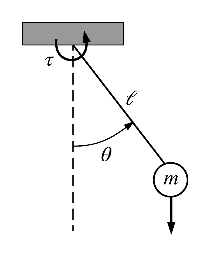
Ejemplo: estabilización péndulo simple
Ejemplo: estabilización péndulo simple
v=-\mathbf{K}\mathbf{z}=-\begin{bmatrix} k_1 & k_2 \end{bmatrix}\begin{bmatrix} z_1 \\ z_2 \end{bmatrix}=-k_1z_1-k_2z_2
u=-\mathbf{K}\left(\mathbf{x}-\mathbf{x}^*\right)+u^*=-\begin{bmatrix} k_1 & k_2 \end{bmatrix}\begin{bmatrix} x_1-\pi \\ x_2-0 \end{bmatrix}+0
u=-k_1(x_1-\pi)-k_2x_2
Procedimiento general: >> ie3041_clase7_procedimiento.mlx
Ejemplo péndulo: >> ie3041_clase7_pendstab.m
Control de alta ganancia
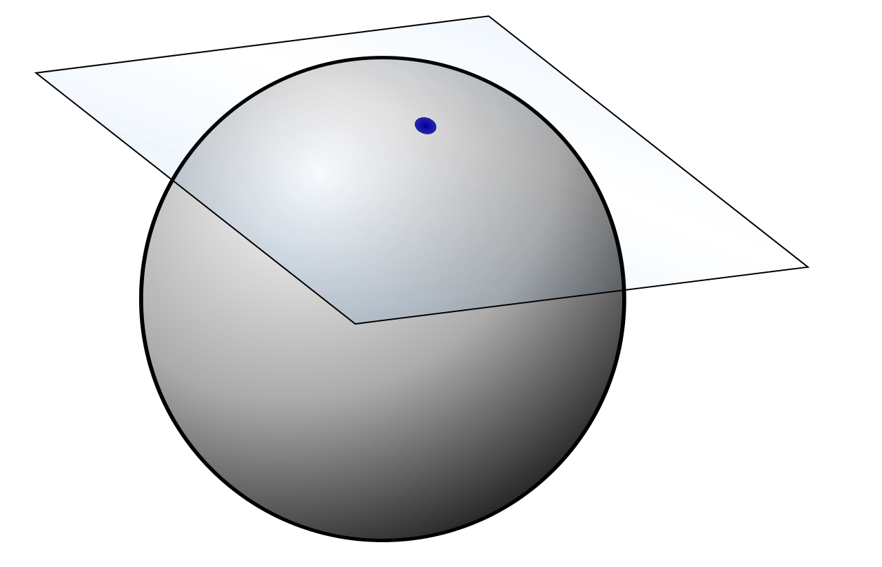
es posible ampliar (hasta el punto que lo permitan los actuadores) la región de atracción del punto de equilibrio u operación a estabilizar, incrementando la ganancia del controlador
\mathbf{u}=-\alpha\mathbf{K}\left(\mathbf{x}-\mathbf{x}_{ss}\right)+\mathbf{u}_{ss}
>> ie3041_clase7_stabilize2d.m
Caso especial para sistemas mecánicos
para el caso especial de sistemas mecánicos completamente actuados y con \(\mathbf{B}\left(\mathbf{q}\right)\) invertible, se tiene que:
\mathbf{u}=-\mathbf{B}^{-1}\left(\mathbf{q}\right)\begin{bmatrix} \mathbf{K}_P & \mathbf{K}_D \end{bmatrix} \begin{bmatrix} \mathbf{q}-\mathbf{q}_{ss} \\ \dot{\mathbf{q}} \end{bmatrix}
+\mathbf{B}^{-1}\left(\mathbf{q}\right)\mathbf{G}\left(\mathbf{q}\right)
estabiliza el punto \(\left(\mathbf{q}_{ss},\mathbf{0}\right)\) del sistema mecánico
Control PD para sistemas mecánicos
para el caso especial de sistemas mecánicos completamente actuados y con \(\mathbf{B}\left(\mathbf{q}\right)\) invertible, se tiene que:
\mathbf{u}=-\mathbf{B}^{-1}\left(\mathbf{q}\right)\begin{bmatrix} \mathbf{K}_P & \mathbf{K}_D \end{bmatrix} \begin{bmatrix} \mathbf{q}-\mathbf{q}_{ss} \\ \dot{\mathbf{q}} \end{bmatrix}
+\mathbf{B}^{-1}\left(\mathbf{q}\right)\mathbf{G}\left(\mathbf{q}\right)
estabiliza el punto \(\left(\mathbf{q}_{ss},\mathbf{0}\right)\) del sistema mecánico
\mathbf{K}\left(\mathbf{q}\right)
\mathbf{x}-\mathbf{x}_{ss}
\mathbf{u}_{ss}(\mathbf{q})
\succ 0
Control PD para sistemas mecánicos
IE3041 - Lecture 7 (2025)
By Miguel Enrique Zea Arenales


