Introducción al control óptimo
IE3041 - Sistemas de Control 2

¿Dónde estamos por el momento?
condición inicial \(\mathbf{x}_0\)
"meta" \(\mathbf{x}_{ss}\)
¿Dónde estamos por el momento?
condición inicial \(\mathbf{x}_0\)
"meta" \(\mathbf{x}_{ss}\)
control LTI local
\(\mathbf{x}_0\) debe de estar dentro de la región de atracción para que funcione
¿Dónde estamos por el momento?
condición inicial \(\mathbf{x}_0\)
"meta" \(\mathbf{x}_{ss}\)
control LTI local
\(\mathbf{x}_0\) debe de estar dentro de la región de atracción para que funcione
¿Dónde estamos por el momento?
condición inicial \(\mathbf{x}_0\)
"meta" \(\mathbf{x}_{ss}\)
control LTI local
\(\mathbf{x}_0\) debe de estar dentro de la región de atracción para que funcione
¿Dónde estamos por el momento?
condición inicial \(\mathbf{x}_0\)
"meta" \(\mathbf{x}_{ss}\)
control LTI de alta ganancia?
¿Dónde estamos por el momento?
condición inicial \(\mathbf{x}_0\)
"meta" \(\mathbf{x}_{ss}\)
control LTI de alta ganancia?
\(\Rightarrow\) puede requerir demasiado esfuerzo de control
¿Dónde estamos por el momento?
condición inicial \(\mathbf{x}_0\)
"meta" \(\mathbf{x}_{ss}\)
estrategias como gain-scheduling?
¿Dónde estamos por el momento?
condición inicial \(\mathbf{x}_0\)
"meta" \(\mathbf{x}_{ss}\)
estrategias como gain-scheduling?
\(\Rightarrow\) asumen una visión demasiado LTI de la realidad (?)
¿Dónde estamos por el momento?
el problema con estas estrategias es que son sólo "decentes" a pesar de requerir una gran cantidad de manipulaciones matemáticas
¿Dónde estamos por el momento?
el problema con estas estrategias es que son sólo "decentes" a pesar de requerir una gran cantidad de manipulaciones matemáticas
esta visión local del mundo impide que el controlador explote la dinámica del sistema
¿Dónde estamos por el momento?
el problema con estas estrategias es que son sólo "decentes" a pesar de requerir una gran cantidad de manipulaciones matemáticas
esta visión local del mundo impide que el controlador explote la dinámica del sistema
¿Qué estamos buscando?
¿Dónde estamos por el momento?
condición inicial \(\mathbf{x}_0\)
"meta" \(\mathbf{x}_{ss}\)
¿Dónde estamos por el momento?
condición inicial \(\mathbf{x}_0\)
"meta" \(\mathbf{x}_{ss}\)
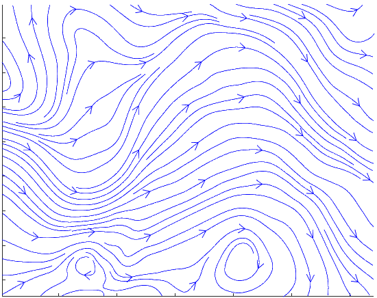
¿Dónde estamos por el momento?
condición inicial \(\mathbf{x}_0\)
"meta" \(\mathbf{x}_{ss}\)
se aprovecha el flujo para una estrategia más eficiente
¿Dónde estamos por el momento?
condición inicial \(\mathbf{x}_0\)
"meta" \(\mathbf{x}_{ss}\)
se aprovecha el flujo para una estrategia más eficiente
óptima
\(\Rightarrow\) control óptimo
¿Dónde estamos por el momento?
Control óptimo
problema de control formulado como búsqueda
similar a los casos de optimización "simples", el control óptimo busca resolver un problema específico de optimización pero más complejo | abstracto
Control óptimo
problema de control formulado como búsqueda
la solución es una trayectoria específica, por lo que el problema también se conoce como optimización de trayectorias
similar a los casos de optimización "simples", el control óptimo busca resolver un problema específico de optimización pero más complejo | abstracto
Control óptimo
problema de control formulado como búsqueda
\begin{aligned}
\mathbf{u}^\star(t) = & \displaystyle\arg\min_{\mathbf{u(t)}} \displaystyle\int_{t_0}^{t_f} \mathcal{L}\left(\mathbf{x}(\tau), \mathbf{u}(\tau) \right)d\tau + \varphi\left(\mathbf{x}_0,\mathbf{x}_f\right) \\
& \textrm{s.t.} \quad \dot{\mathbf{x}}=\mathbf{f}\left(\mathbf{x}, \mathbf{u}\right) \\
\end{aligned}
El problema de control óptimo
\begin{aligned}
\mathbf{u}^\star(t) = & \displaystyle\arg\min_{\mathbf{u(t)}} \displaystyle\int_{t_0}^{t_f} \mathcal{L}\left(\mathbf{x}(\tau), \mathbf{u}(\tau) \right)d\tau + \varphi\left(\mathbf{x}_0,\mathbf{x}_f\right) \\
& \textrm{s.t.} \quad \dot{\mathbf{x}}=\mathbf{f}\left(\mathbf{x}, \mathbf{u}\right) \\
\end{aligned}
\(=J\left(\mathbf{u}(t)\right)\) funcional de costo
El problema de control óptimo
\begin{aligned}
\mathbf{u}^\star(t) = & \displaystyle\arg\min_{\mathbf{u(t)}} \displaystyle\int_{t_0}^{t_f} \mathcal{L}\left(\mathbf{x}(\tau), \mathbf{u}(\tau) \right)d\tau + \varphi\left(\mathbf{x}_0,\mathbf{x}_f\right) \\
& \textrm{s.t.} \quad \dot{\mathbf{x}}=\mathbf{f}\left(\mathbf{x}, \mathbf{u}\right) \\
\end{aligned}
horizonte finito
El problema de control óptimo
\begin{aligned}
\mathbf{u}^\star(t) = & \displaystyle\arg\min_{\mathbf{u(t)}} \displaystyle\int_{t_0}^{t_f} \mathcal{L}\left(\mathbf{x}(\tau), \mathbf{u}(\tau) \right)d\tau + \varphi\left(\mathbf{x}_0,\mathbf{x}_f\right) \\
& \textrm{s.t.} \quad \dot{\mathbf{x}}=\mathbf{f}\left(\mathbf{x}, \mathbf{u}\right) \\
\end{aligned}
\mathbf{x_0} \\
t_0
\mathbf{x_f} \\
t_f
costo de parqueo o de frontera
costo de trayectoria
El problema de control óptimo
\begin{aligned}
\mathbf{u}^\star(t) = & \displaystyle\arg\min_{\mathbf{u(t)}} \displaystyle\int_{t_0}^{t_f} \mathcal{L}\left(\mathbf{x}(\tau), \mathbf{u}(\tau) \right)d\tau + \varphi\left(\mathbf{x}_0,\mathbf{x}_f\right) \\
& \textrm{s.t.} \quad \dot{\mathbf{x}}=\mathbf{f}\left(\mathbf{x}, \mathbf{u}\right) \\
\end{aligned}
obliga que la solución cumpla con la dinámica del sistema
El problema de control óptimo
1. ¿Variables de decisión?
¿Por qué es complicado este problema?
\dim(\mathbf{u})=m
1. ¿Variables de decisión?
¿Por qué es complicado este problema?
\dim(\mathbf{u})=m
\dim\left(\mathbf{u}(t)\right)=
\dim\left( \begin{bmatrix} u_1(t) \\ u_2(t) \\ \vdots \\ u_m(t)\end{bmatrix} \right)
1. ¿Variables de decisión?
¿Por qué es complicado este problema?
\dim(\mathbf{u})=m
\dim\left(\mathbf{u}(t)\right)=
\dim\left( \begin{bmatrix} u_1(t) \\ u_2(t) \\ \vdots \\ u_m(t)\end{bmatrix} \right)
=\dim\left(u_1(t)\right)+\dim\left(u_2(t)\right)+\cdots+\dim\left(u_m(t)\right)
1. ¿Variables de decisión?
¿Por qué es complicado este problema?
\dim(\mathbf{u})=m
\dim\left(\mathbf{u}(t)\right)=
\dim\left( \begin{bmatrix} u_1(t) \\ u_2(t) \\ \vdots \\ u_m(t)\end{bmatrix} \right)
=\dim\left(u_1(t)\right)+\dim\left(u_2(t)\right)+\cdots+\dim\left(u_m(t)\right)
señales de tiempo continuo \(\Rightarrow \dim \to \infty\)
1. ¿Variables de decisión?
¿Por qué es complicado este problema?
\dim(\mathbf{u})=m
\dim\left(\mathbf{u}(t)\right)=
\dim\left( \begin{bmatrix} u_1(t) \\ u_2(t) \\ \vdots \\ u_m(t)\end{bmatrix} \right)
=\dim\left(u_1(t)\right)+\dim\left(u_2(t)\right)+\cdots+\dim\left(u_m(t)\right) \\
=m \times \infty = \infty
(!)
1. ¿Variables de decisión?
¿Por qué es complicado este problema?
2. Resticciones
\textrm{s.t.} \quad \dot{\mathbf{x}}=\mathbf{f}\left(\mathbf{x}, \mathbf{u}\right)
restricción de igualdad en forma de una ecuación diferencial vectorial no lineal
¿Por qué es complicado este problema?
2. Resticciones
¿Por qué es complicado este problema?
\textrm{s.t.} \quad \dot{\mathbf{x}}=\mathbf{f}\left(\mathbf{x}, \mathbf{u}\right)
restricción de igualdad en forma de una ecuación diferencial vectorial no lineal
(!)
-
analíticas
- cálculo de variaciones
- teoría de Hamilton-Jacobi-Bellman (dynamic programming)
- principio del máximo de Pontryagin
-
numéricas
- requieren transcripción a un programa no lineal
¿Qué herramientas existen para resolver?
-
analíticas
- cálculo de variaciones
- teoría de Hamilton-Jacobi-Bellman (dynamic programming)
- principio del máximo de Pontryagin
-
numéricas
- requieren transcripción a un programa no lineal
¿Qué herramientas existen para resolver?
\begin{aligned}
& \displaystyle\min_{\mathbf{u(t)}} \displaystyle\int_{t_0}^{t_f} \mathcal{L}\left(\mathbf{x}(\tau), \mathbf{u}(\tau) \right)d\tau + \varphi\left(\mathbf{x}_0,\mathbf{x}_f\right) \\
& \textrm{s.t.} \quad \dot{\mathbf{x}}=\mathbf{f}\left(\mathbf{x}, \mathbf{u}\right) \\
\end{aligned}
Transcripción directa
\begin{aligned}
& \displaystyle\min_{\mathbf{u(t)}} \displaystyle\int_{t_0}^{t_f} \mathcal{L}\left(\mathbf{x}(\tau), \mathbf{u}(\tau) \right)d\tau + \varphi\left(\mathbf{x}_0,\mathbf{x}_f\right) \\
& \textrm{s.t.} \quad \dot{\mathbf{x}}=\mathbf{f}\left(\mathbf{x}, \mathbf{u}\right) \\
\end{aligned}
\begin{aligned}
& \displaystyle\min_{\mathbf{z}} & f\left(\mathbf{z}\right) \qquad \\
& \text{s.t.} & \mathbf{g}_i\left(\mathbf{z}\right) \le\mathbf{0} \quad \forall i \\
& & \mathbf{h}_j\left(\mathbf{z}\right)=\mathbf{0} \quad \forall j
\end{aligned}
primero discretizamos y luego optimizamos
Transcripción directa
sencillos de plantear y resolver pero menos precisos
Transcripción directa
sencillos de plantear y resolver pero menos precisos
¿Transcripción indirecta?
presentan mejor precisión pero requieren de las técnicas analíticas para su planteamiento
Transcripción directa
sencillos de plantear y resolver pero menos precisos
¿Transcripción indirecta?
presentan mejor precisión pero requieren de las técnicas analíticas para su planteamiento
\(\Rightarrow\) NO los emplearemos
Transcripción directa
-
métodos de disparo (shooting)
- basados en simulación
- buenos para problemas sin (muchas) restricciones
-
métodos de colocación (collocation)
- basados en aproximaciones de la dinámica
- mejores para problemas con restricciones
Dos métodos
Shooting vs Collocation
-
métodos de disparo (shooting)
- basados en simulación
- buenos para problemas sin (muchas) restricciones
-
métodos de colocación (collocation)
- basados en aproximaciones de la dinámica
- mejores para problemas con restricciones
método de colocación directa
Dos métodos
Optimización de trayectorias mediante colocación directa
El método de colocación directa
\begin{aligned}
& \displaystyle\min_{t_0,t_f,\mathbf{x(t)},\mathbf{u(t)}} \ \ \displaystyle\int_{t_0}^{t_f} \mathcal{L}\left(\tau, \mathbf{x}(\tau), \mathbf{u}(\tau) \right)d\tau + \varphi\left(t_0,t_f,\mathbf{x}_0,\mathbf{x}_f\right) \\
& \qquad \textrm{s.t.} \qquad \dot{\mathbf{x}}(t)=\mathbf{f}\left(t,\mathbf{x}(t), \mathbf{u}(t)\right) \qquad \\
& \qquad \qquad \quad \ \mathbf{h}\left(t, \mathbf{x}(t), \mathbf{u}(t)\right) \le \mathbf{0} \\
& \qquad \qquad \quad \ \mathbf{g}\left(t_0, t_f, \mathbf{x}_0, \mathbf{x}_f\right) \le \mathbf{0} \\
& \qquad \qquad \quad \ \mathbf{x}_\mathrm{low} \le \mathbf{x}(t) \le \mathbf{x}_\mathrm{upp} \\
& \qquad \qquad \quad \ \mathbf{u}_\mathrm{low} \le \mathbf{u}(t) \le \mathbf{u}_\mathrm{upp} \\
& \qquad \qquad \quad \ t_\mathrm{low} \le t_0 \le t_f \le t_\mathrm{upp} \\
& \qquad \qquad \quad \ \mathbf{x}_{0,\mathrm{low}} \le \mathbf{x}_0 \le \mathbf{x}_{0,\mathrm{upp}} \\
& \qquad \qquad \quad \ \mathbf{x}_{f,\mathrm{low}} \le \mathbf{x}_f \le \mathbf{x}_{f,\mathrm{upp}}
\end{aligned}
dynamics constraints
path constraints
boundary constraints
state bounds
control bounds
initial and final time bounds
initial state bounds
final state bounds
Transcribiendo el problema
\displaystyle\min_{t_0,t_f,\mathbf{x(t)},\mathbf{u(t)}}
Variables de decisión
\displaystyle\min_{t_0,t_f,\mathbf{x(t)},\mathbf{u(t)}}
\displaystyle\min_{\mathbf{z}}
Variables de decisión
\mathbf{u}(t)
\mathbf{x}(t)
t
t
t_0
t_f
t_0
t_f
\mathbf{u}(t)
\mathbf{x}(t)
t
t
t_0
t_1
t_2
t_N
\cdots
=t_f
t_0
t_1
t_2
t_N
\cdots
\mathbf{u}(t)
\mathbf{x}(t)
t
t
t_0
t_1
t_2
t_N
\cdots
=t_f
t_0
t_1
t_2
t_N
\cdots
\mathbf{u}(t)
\mathbf{x}(t)
t
t
t_0
t_1
t_2
t_N
\cdots
=t_f
t_0
t_1
t_2
t_N
\cdots
puntos de colocación
\(N\) segmentos
\(M\) puntos de colocación
t \to \left[ t_0, t_1, \cdots, t_N \right], \qquad t_N = t_f \\
\mathbf{u}(t) \to \left[ \mathbf{u}(t_0), \mathbf{u}(t_1), \cdots, \mathbf{u}(t_N) \right] = \left[ \mathbf{u}_0, \mathbf{u}_1, \cdots, \mathbf{u}_N \right] \\
\mathbf{x}(t) \to \left[ \mathbf{x}(t_0), \mathbf{x}(t_1), \cdots, \mathbf{x}(t_N) \right] = \left[ \mathbf{x}_0, \mathbf{x}_1, \cdots, \mathbf{x}_N \right]
\mathbf{x}(t_1)=\mathbf{x}_1=\begin{bmatrix} x_1(t_1) \\ x_2(t_1) \\ \vdots \\ x_n(t_1) \end{bmatrix}
\mathbf{z}=\left[ t_0, t_1, \cdots, t_N, \mathbf{u}_0, \mathbf{u}_1, \cdots, \mathbf{u}_N, \mathbf{x}_0, \mathbf{x}_1, \cdots, \mathbf{x}_N \right]
\mathbf{z}=\left[ t_0, t_1, \cdots, t_N, \mathbf{u}_0, \mathbf{u}_1, \cdots, \mathbf{u}_N, \mathbf{x}_0, \mathbf{x}_1, \cdots, \mathbf{x}_N \right]
\begin{aligned}
t: & \quad M \\
\mathbf{u}(t): & \quad M \times m \\
\mathbf{x}(t): & \quad M \times n \\
\mathbf{z}: & \quad M(n+m+1)
\end{aligned}
variables de decisión
\displaystyle\int_{t_0}^{t_f} \mathcal{L}\left(\tau, \mathbf{x}(\tau), \mathbf{u}(\tau) \right)d\tau + \varphi\left(t_0,t_f,\mathbf{x}_0,\mathbf{x}_f\right)
Función objetivo
\displaystyle\int_{t_0}^{t_f} \mathcal{L}\left(\tau, \mathbf{x}(\tau), \mathbf{u}(\tau) \right)d\tau + \varphi\left(t_0,t_f,\mathbf{x}_0,\mathbf{x}_f\right)
f\left(\mathbf{z}\right)
Función objetivo
\displaystyle\int_{t_0}^{t_f} \mathcal{L}\left(\tau, \mathbf{x}(\tau), \mathbf{u}(\tau) \right)d\tau + \varphi\left(t_0,t_f,\mathbf{x}_0,\mathbf{x}_f\right)
\displaystyle\int_{t_0}^{t_f} \mathcal{L}\left(\tau, \mathbf{x}(\tau), \mathbf{u}(\tau) \right)d\tau + \varphi\left(t_0,t_f,\mathbf{x}_0,\mathbf{x}_f\right)
operador continuo, debe discretizarse
\displaystyle\int_{t_0}^{t_f} \mathcal{L}\left(\tau, \mathbf{x}(\tau), \mathbf{u}(\tau) \right)d\tau + \varphi\left(t_0,t_f,\mathbf{x}_0,\mathbf{x}_f\right)
no hace falta discretizar
operador continuo, debe discretizarse
\displaystyle\int_{t_0}^{t_f} \mathcal{L}\left(\tau, \mathbf{x}(\tau), \mathbf{u}(\tau) \right)d\tau + \varphi\left(t_0,t_f,\mathbf{x}_0,\mathbf{x}_f\right)
no hace falta discretizar
operador continuo, debe discretizarse
\displaystyle\int_{t_0}^{t_f} \mathcal{L}\left(\tau \right)d\tau \approx
collocation method
\displaystyle\int_{t_0}^{t_f} \mathcal{L}\left(\tau, \mathbf{x}(\tau), \mathbf{u}(\tau) \right)d\tau + \varphi\left(t_0,t_f,\mathbf{x}_0,\mathbf{x}_f\right)
no hace falta discretizar
operador continuo, debe discretizarse
\displaystyle\int_{t_0}^{t_f} \mathcal{L}\left(\tau \right)d\tau \approx
- trapezoidal
- Hermite-Simpson
- Runge-Kutta
- Chebyshev
- ...
collocation method
\displaystyle\int_{t_0}^{t_f} \mathcal{L}\left(\tau, \mathbf{x}(\tau), \mathbf{u}(\tau) \right)d\tau + \varphi\left(t_0,t_f,\mathbf{x}_0,\mathbf{x}_f\right)
no hace falta discretizar
operador continuo, debe discretizarse
\displaystyle\int_{t_0}^{t_f} \mathcal{L}\left(\tau \right)d\tau \approx
- trapezoidal (ejemplo)
- Hermite-Simpson
- Runge-Kutta
- Chebyshev
- ...
collocation method
\displaystyle\int_{t_0}^{t_f} \mathcal{L}\left(\tau \right)d\tau \approx
\displaystyle\sum_{k=0}^{N-1} \dfrac{h_k}{2}\left(\mathcal{L}_k+\mathcal{L}_{k+1}\right)
\displaystyle\int_{t_0}^{t_f} \mathcal{L}\left(\tau \right)d\tau \approx
\displaystyle\sum_{k=0}^{N-1} \dfrac{h_k}{2}\left(\mathcal{L}_k+\mathcal{L}_{k+1}\right)
\mathcal{L}_k=\mathcal{L}\left(t_k,\mathbf{x}_k,\mathbf{u}_k\right)
h_k = \Delta t \\
h_k \to \left[h_1,\cdots,h_N\right]
paso fijo
paso variable, las \(h_k\) deben añadirse a las variables de decisión
el tipo de colocación también informa sobre la interpolación a emplear para \(\mathbf{u}(t)\)
\textrm{s.t.} \quad \dot{\mathbf{x}}(t)=\mathbf{f}\left(t,\mathbf{x}(t), \mathbf{u}(t)\right)
Restricción de dinámica
\textrm{s.t.} \quad \dot{\mathbf{x}}(t)=\mathbf{f}\left(t,\mathbf{x}(t), \mathbf{u}(t)\right)
\textrm{s.t.} \quad \mathbf{h}\left(\mathbf{z}\right)=\mathbf{0}
Restricción de dinámica
\dot{\mathbf{x}}(t)=\mathbf{f}\left(t,\mathbf{x}(t), \mathbf{u}(t)\right) \\
\displaystyle\int_{t_k}^{t_{k+1}} \dot{\mathbf{x}}(\tau)d\tau=\displaystyle\int_{t_k}^{t_{k+1}} \mathbf{f}\left(\tau,\mathbf{x}(\tau), \mathbf{u}(\tau)\right)d\tau
\dot{\mathbf{x}}(t)=\mathbf{f}\left(t,\mathbf{x}(t), \mathbf{u}(t)\right) \\
\displaystyle\int_{t_k}^{t_{k+1}} \dot{\mathbf{x}}(\tau)d\tau=\displaystyle\int_{t_k}^{t_{k+1}} \mathbf{f}\left(\tau,\mathbf{x}(\tau), \mathbf{u}(\tau)\right)d\tau
\mathbf{x}_{k+1}-\mathbf{x}_k=\displaystyle\int_{\Delta t} \mathbf{f}\left(\tau,\mathbf{x}(\tau), \mathbf{u}(\tau)\right)d\tau \approx
de nuevo depende del método de colocación
\mathbf{x}_{k+1}-\mathbf{x}_k=\displaystyle\int_{\Delta t} \mathbf{f}\left(\tau,\mathbf{x}(\tau), \mathbf{u}(\tau)\right)d\tau \approx
\dfrac{h_k}{2}\left(\mathbf{f}_{k+1}+\mathbf{f}_k\right)
ej: colocación trapezoidal
\mathbf{x}_{k+1}-\mathbf{x}_k=\displaystyle\int_{\Delta t} \mathbf{f}\left(\tau,\mathbf{x}(\tau), \mathbf{u}(\tau)\right)d\tau \approx
\dfrac{h_k}{2}\left(\mathbf{f}_{k+1}+\mathbf{f}_k\right)
ej: colocación trapezoidal
\mathbf{f}_k=\mathbf{f}\left(t_k, \mathbf{x}_k, \mathbf{u}_k\right)
\mathbf{x}_{k+1}-\mathbf{x}_k=\displaystyle\int_{\Delta t} \mathbf{f}\left(\tau,\mathbf{x}(\tau), \mathbf{u}(\tau)\right)d\tau \approx
\dfrac{h_k}{2}\left(\mathbf{f}_{k+1}+\mathbf{f}_k\right)
ej: colocación trapezoidal
\mathbf{f}_k=\mathbf{f}\left(t_k, \mathbf{x}_k, \mathbf{u}_k\right)
\Rightarrow \mathbf{h}_i\left(\mathbf{z}\right): \quad
\mathbf{x}_{k+1}-\mathbf{x}_k-\dfrac{h_k}{2}\left(\mathbf{f}_{k+1}+\mathbf{f}_k\right)=\mathbf{0}, \ i=1,\cdots,N
(restricciones de colocación)
el resto de restricciones se transcriben tal cual (dado que ya están planteadas de forma discreta)
el resto de restricciones se transcriben tal cual (dado que ya están planteadas de forma discreta)
finalmente, se recomienda como aproximación inicial:
\mathbf{u}^0(t)=\mathbf{0}
el resto de restricciones se transcriben tal cual (dado que ya están planteadas de forma discreta)
finalmente, se recomienda como aproximación inicial:
\mathbf{u}^0(t)=\mathbf{0}
\mathbf{x}^0(t)=\mathbf{x}_0\left(1-t/t_f\right) + \mathbf{x}_f\left(t/t_f\right)
(interpolación lineal entre \(\mathbf{x}_0\) y \(\mathbf{x}_f\))
Ya con esto podemos plantear el problema como un programa no lineal y emplear (por ejemplo):
z = fmincon(fun, z0, A, b, Aeq, beq, lb, ub, nonlcon)Resolviendo el problema
Ya con esto podemos plantear el problema como un programa no lineal y emplear (por ejemplo):
z = fmincon(fun, z0, A, b, Aeq, beq, lb, ub, nonlcon)Resolviendo el problema
Ejemplo: cart-pole swing up
Ejemplo: cart-pole swing up
Desde cero
>> ie3041_clase12_cartpole_manual_solve.m
Con OptimTraj
>> ie3041_clase12_cartpole_optimtraj_solve.m
Simulación de resultados
>> ie3041_clase12_cartpole_sim.m
IE3041 - Lecture 12 (2025)
By Miguel Enrique Zea Arenales


