Shifts in Demand Curves; Elasticity of Demand
Christopher Makler
Stanford University Department of Economics
Econ 50: Lecture 9
pollev.com/chrismakler

How are you feeling on the material so far?
Quick note: I haven't had time to write up lecture notes for Monday, because they involve graphs I haven't yet produced!


Read "Slutsky Equation" from Varian; any edition will do.
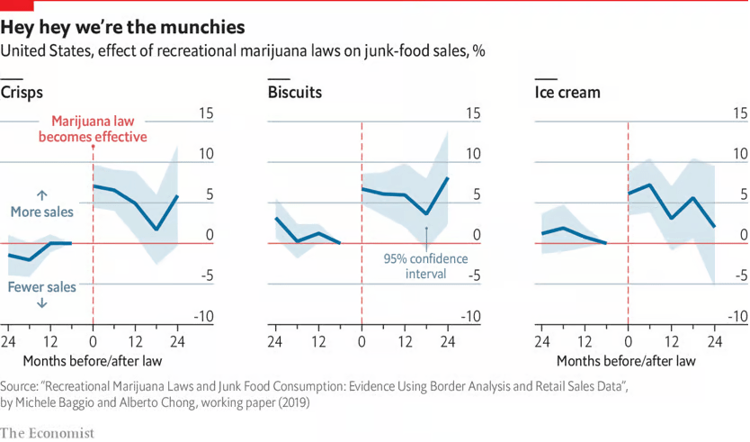
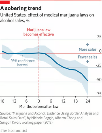
What does this imply about complements and substitutes for marijuana?
Remember what you learned about demand and demand curves in Econ 1 / high school:
- The demand curve shows the quantity demanded of a good at different prices
- A change in the price of a good results in a movement along its demand curve
- A change in income or the price of other goods results in a shift of the demand curve
-
- If two goods are substitutes, an increase in the price of one will increase the demand for the other (shift the demand curve to the right).
- If two goods are complements, an increase in the price of one will decrease the demand for the other (shift the demand curve to the left).
- If a good is a normal good, an increase in income will increase demand for the good
- If a good is an inferior good, an increase in income will decrease demand the good
x_1^*(p_1,p_2,m)\ \
Three Relationships
...its own price changes?
Movement along the demand curve
...the price of another good changes?
Complements
Substitutes
Independent Goods
How does the quantity demanded of a good change when...
...income changes?
Normal goods
Inferior goods
Giffen goods
(possible) shift of the demand curve
x_1^*(p_1,p_2,m)\ \
Three Relationships
...its own price changes?
Movement along the demand curve
How does the quantity demanded of a good change when...
The demand curve for a good
shows the quantity demanded of that good
as a function of its own price
holding all other factors constant
(ceteris paribus)
x_1
x_1
x_2
p_1
DEMAND CURVE FOR GOOD 1
BL_{p_1 = 2}
BL_{p_1 = 3}
BL_{p_1 = 4}
2
3
4
"Good 1 - Good 2 Space"
"Quantity-Price Space for Good 1"
BL
x_1^*(p_1,p_2,m)\ \
Three Relationships
...the price of another good changes?
How does the quantity demanded of a good change when...
Substitutes
Complements
When the price of one good goes up, demand for the other increases.
When the price of one good goes up, demand for the other decreases.


Independent
Demand not related
x_1
x_2
x_1
x_2
Complements: \(p_2 \uparrow \Rightarrow x_1^* \downarrow\)
What happens to the quantity of good 1 demanded when the price of good 2 increases?
Substitutes: \(p_2 \uparrow \Rightarrow x_1^* \uparrow\)
pollev.com/chrismakler
Goods are complements if which of the following would cause a RIGHTWARD shift in the demand curve for good 1?
An increase in the price of good 2
A decrease in the price of good 2
An increase in income
A decrease in income
x_1^*(p_1,p_2,m)\ \
Three Relationships
...its own price changes?
Movement along the demand curve
...the price of another good changes?
Complements
Substitutes
Independent Goods
How does the quantity demanded of a good change when...
...income changes?
Normal goods
Inferior goods
Giffen goods
(possible) shift of the demand curve
x_1^*(p_1,p_2,m)\ \
Three Relationships
How does the quantity demanded of a good change when...
...income changes?
Normal Goods
Inferior Goods
When your income goes up,
demand for the good increases.
When your income goes up,
demand for the good decreases.


The income offer curve shows how the optimal bundle changes in good 1-good 2 space as income changes.
x_1
x_2
x_1
x_2
Good 1 normal: \(m \uparrow \Rightarrow x_1^* \uparrow\)
What happens to the quantity of good 1 demanded when the income increases?
Good 1 inferior: \(m \uparrow \Rightarrow x_1^* \downarrow\)
pollev.com/chrismakler
The "rule" for Cobb-Douglas is that you spend a certain fraction of your income on each good, regardless of prices or income.
What does this make the two goods?
Complements
Substitutes
Normal
Inferior
CES Utility
= \begin{cases}\infty & \text{ if } x_1 < x_2 \\ 0 & \text{ if } x_1 > x_2 \end{cases}
-\infty
1
0
MRS = \left(x_2 \over x_1\right)^\infty
MRS = {x_2 \over x_1}
MRS = 1
r
u(x_1,x_2) = \min\{x_1,x_2\}
u(x_1,x_2) = x_1x_2
u(x_1,x_2) = x_1 + x_2
PERFECT
SUBSTITUTES
PERFECT
COMPLEMENTS
INDEPENDENT
PERFECT
SUBSTITUTES
u(x_1,x_2) = (x_1^r+x_2^r)^{1 \over r}
Constant Elasticity of Substitution (CES) Utility
MRS = \left(x_2 \over x_1\right)^{1-r}
[50Q only]
u(x_1,x_2) = (x_1^r+x_2^r)^{1 \over r}
Constant Elasticity of Substitution (CES) Utility
MRS = \left(x_2 \over x_1\right)^{1-r}
-\infty
1
r
COMPLEMENTS: \(r < 0\)
SUBSTITUTES: \(r > 0\)
-1
MRS = \left(x_2 \over x_1\right)^2
{1 \over 2}
MRS = \left(x_2 \over x_1\right)^{1 \over 2}
u(x_1,x_2) = (x_1^{-1}+x_2^{-1})^{-1}
u(x_1,x_2) = \left(x_1^{1 \over 2} + x_2^{1 \over 2}\right)^2
- A change in the price of a good results in a movement along its demand curve
- A change in income or the price of other goods results in a shift of the demand curve
Elasticity
Why Elasticity?

Notation
\epsilon_{Y,X} = \frac{\% \Delta Y}{\% \Delta X}
\text{Elasticity }(\epsilon) = \frac{\% \text{ change in endogenous variable}}{\% \text{ change in exogenous variable}}
"X elasticity of Y"
or "Elasticity of Y with respect to X"
Examples:
"Price elasticity of demand"
"Income elasticity of demand"
"Cross-price elasticity of demand"
"Price elasticity of supply"
Perfectly Inelastic
Inelastic
Unit Elastic
Elastic
Perfectly Elastic
|\epsilon| = 0
|\epsilon| < 1
|\epsilon| = 1
|\epsilon| > 1
|\epsilon| = \infty
Doesn't change
Changes by less than the change in X
Changes proportionally to the change in X
Changes by more than the change in X
Changes "infinitely" (usually: to/from zero)
How does the endogenous variable Y respond to a
change in the exogenous variable X?
\text{Elasticity }(\epsilon) = \frac{\% \text{ change in endogenous variable}}{\% \text{ change in exogenous variable}}
(note: all of these refer to the ratio of the perentage change, not absolute change)
Own-Price Elasticity
What is the effect of a 1% change
in the price of good 1 \((p_1)\) on the quantity demanded of good 1 \((x_1^*)\)?
no change
perfectly inelastic
less than 1%
inelastic
exactly 1%
unit elastic
more than 1%
elastic
-
How does \(x_1^*\) change with \(p_1\)?
- Own-price elasticity
- Elastic vs. inelastic
x_1^*(p_1,p_2,m)
Three Relationships
Cross-Price Elasticity
What is the effect of an increase
in the price of good 2 \((p_2)\) on the quantity demanded of good 1 \((x_1^*)\)?
no change
independent
decrease
complements
increase
substitutes
-
How does \(x_1^*\) change with \(p_1\)?
- Own-price elasticity
- Elastic vs. inelastic
-
How does \(x_1^*\) change with \(p_2\)?
- Cross-price elasticity
- Complements vs. substitutes
x_1^*(p_1,p_2,m)
Three Relationships
Income Elasticity
What is the effect of an increase
in income \((m)\) on the quantity demanded of good 1 \((x_1^*)\)?
decrease
good 1 is inferior
increase
good 1 is normal
-
How does \(x_1^*\) change with \(p_1\)?
- Own-price elasticity
- Elastic vs. inelastic
-
How does \(x_1^*\) change with \(p_2\)?
- Cross-price elasticity
- Complements vs. substitutes
-
How does \(x_1^*\) change with \(m\)?
- Income elasticity
- Normal vs. inferior goods
x_1^*(p_1,p_2,m)
Three Relationships
Calculating Elasticities in General
\epsilon_{Y,X}
= \frac{\% \Delta Y}{\% \Delta X}
= \frac{\Delta Y / Y}{\Delta X / X}
= \frac{\Delta Y}{\Delta X}\times \frac{X}{Y}
\text{Suppose }Y \text{ is a function of }X.
General formula:
Linear relationship:
Using calculus:
Multiplicative relationship:
Y = mX + b
Y = f(X)
Y = aX^b
\epsilon_{y,x}
= \frac{\% \Delta y}{\% \Delta x}
= \frac{\Delta y / y}{\Delta x / x}
= \frac{\Delta y}{\Delta x}\times \frac{x}{y}
\text{Suppose }y \text{ is a function of }x.
\text{In the limit, as }\Delta x \rightarrow 0:
\epsilon_{y,x} = \frac{dy}{dx}\times \frac{x}{y}
Demand Elasticity:
\(\epsilon_{q,p} = \frac{\%\Delta q}{\%\Delta p}\)
\epsilon_{q,p} = \frac{dq}{dp}\times \frac{p}{q}
\text{General formula: }\epsilon_{Y,X} = \frac{\Delta Y}{\Delta X}\times \frac{X}{Y}
\text{If }Y = a + bX \text{, then }\frac{\Delta Y}{\Delta X} =
b
\epsilon_{Y,X} = b\times \frac{X}{a + bX}
Note: the slope of the relationship is \(b\).
Elasticity is related to, but not the same thing as, slope.
= \frac{bX}{a + bX}
\epsilon_{y,x}
= \frac{\% \Delta y}{\% \Delta x}
= \frac{\Delta y / y}{\Delta x / x}
= \frac{\Delta y}{\Delta x}\times \frac{x}{y}
\text{Suppose }y \text{ is a function of }x.
\text{In the limit, as }\Delta x \rightarrow 0:
\epsilon_{y,x} = \frac{dy}{dx}\times \frac{x}{y}
\text{General formula: }\epsilon_{y,x} = \frac{dy}{dx}\times \frac{x}{y}
\text{If }y = ax^b \text{, then }\frac{dy}{dx} =
abx^{b-1}
\epsilon_{y,x} = abx^{b-1} \times \frac{x}{ax^b}
= b
This is related to logs...let's go to the board for that though. :)
This is a super useful trick and one that comes up on midterms all the time!
Next week: finish with tradeoffs
(for now)
Monday
What makes things complements or substitutes?
Income and substitution effects of a price change
(Varian reading)
Wednesday
Cost minimization, as opposed to utility maximization...
which will lead us to the theory of the firm.
ON HW 3 AND MIDTERM
NOT ON MIDTERM BUT IMPORTANT!
I have office hours today
from 1-3 in Econ 106. Come!
Econ 50 | Spring 25 | Lecture 9
By Chris Makler


