Decomposing a Price Change into Income and Substitution Effects
Christopher Makler
Stanford University Department of Economics
Econ 50: Lecture 10
Solving Climate Change in one Easy Step
- Climate change is real and caused in large part by burning fossil fuels.
- Transportation is a big part of the problem.
- A higher tax on gasoline would make people drive less, and have many other benefits. See Mankiw's Pigou Club Manifesto.
- Estimates vary, but $10/gallon seems about right.
but...
$10/gallon gas would hurt a lot of people, especially those with lower incomes who depend on a car to get to work
Can we give them a certain amount of money that would make them no worse off than they were before, to compensate them for the price increase?


Remember what you learned about demand and demand curves in Econ 1 / high school:
- The demand curve shows the quantity demanded of a good at different prices
- A change in the price of a good results in a movement along its demand curve
- A change in income or the price of other goods results in a shift of the demand curve
-
- If two goods are substitutes, an increase in the price of one will increase the demand for the other (shift the demand curve to the right).
- If two goods are complements, an increase in the price of one will decrease the demand for the other (shift the demand curve to the left).
- If a good is a normal good, an increase in income will increase demand for the good
- If a good is an inferior good, an increase in income will decrease demand the good
x_1^*(p_1,p_2,m)\ \
Three Relationships
...its own price changes?
Movement along the demand curve
...the price of another good changes?
Complements
Substitutes
Independent Goods
How does the quantity demanded of a good change when...
...income changes?
Normal goods
Inferior goods
Giffen goods
(possible) shift of the demand curve
x_1^*(p_1,p_2,m)\ \
Three Relationships
...the price of another good changes?
How does the quantity demanded of a good change when...
Substitutes
Complements
When the price of one good goes up, demand for the other increases.
When the price of one good goes up, demand for the other decreases.


Independent
Demand not related
x_1
x_2
x_1
x_2
Complements: \(p_2 \uparrow \Rightarrow x_1^* \downarrow\)
What happens to the quantity of good 1 demanded when the price of good 2 increases?
Substitutes: \(p_2 \uparrow \Rightarrow x_1^* \uparrow\)
x_1^*(p_1,p_2,m)\ \
Three Relationships
How does the quantity demanded of a good change when...
...income changes?
Normal Goods
Inferior Goods
When your income goes up,
demand for the good increases.
When your income goes up,
demand for the good decreases.


The income offer curve shows how the optimal bundle changes in good 1-good 2 space as income changes.
x_1
x_2
x_1
x_2
Good 1 normal: \(m \uparrow \Rightarrow x_1^* \uparrow\)
What happens to the quantity of good 1 demanded when the income increases?
Good 1 inferior: \(m \uparrow \Rightarrow x_1^* \downarrow\)
Demand function: how does an optimal bundle change when prices or income changes?
If we want to know how best to implement a policy, we want to know why it changes.
For example: we could be interested in how far a cannonball travels, so we can aim it at a target.
To do this, a physicist would decompose its velocity
into the horizontal portion and vertical portion:
Two Effects
Substitution Effect
Effect of change in relative prices, holding purchasing power constant.
Effect of change in real income,
holding relative prices constant.
Income Effect
Decomposition Bundle
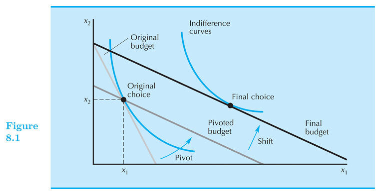
Suppose that, after a price change,
we adjusted the consumer's income
so that they had exactly the amount of money needed to afford their initial bundle \(X\)?
Approach
TOTAL EFFECT
X
Z
Y
INITIAL BUNDLE
FINAL BUNDLE
DECOMPOSITION BUNDLE
SUBSTITUTION EFFECT
INCOME EFFECT
Slutsky Decomposition
Let's think about an increase in the price of good 1.
X
\(BL_1\)
\(BL_2\)
We start out at bundle X.
The price of good 1 increases, pivoting the budget line in.
Z
The new optimal bundle is Z.
Slutsky Decomposition
X
Y
\(BL_1\)
\(BL_2\)
Now suppose we had given the consumer just enough income to afford their original bundle \(X\) at the new price.
DECOMPOSITION BUDGET LINE \(BL_D\)
Z
This "decompensation budget line" would have the same slope as \(BL_2\), but pass through bundle \(X\).
We call the point the consumer would have bought with this budget line the Slutsky Decomposition Bundle \(Y\)
SUBSTITUTION EFFECT
INCOME EFFECT
Substitution effect: \(X \rightarrow Y\)
Income effect: \(Y \rightarrow Z\)
Slutsky Decomposition
X
\(BL_1\)
\(BL_2\)
One way to think about this decomposition is that the budget line "pivots" around the point \(X\),
and then "shifts" inward.
DECOMPOSITION BUDGET LINE \(BL_D\)
The pivot captures the change in the relative price, but keeps the purchasing power the same: you can still (just) afford \(X\).
The shift captures the change in real purchasing power, holding the price ratio constant (parallel shift)
Slutsky Decomposition
X
\(BL_1\)
\(TC_1\)
Let's think of this now in terms of the tangency condition.
Think about the Cobb-Douglas utility function
u(x_1,x_2) = x_1x_2
MRS = {p_1 \over p_2}
MRS = {x_2 \over x_1}
Tangency condition
x_2 = {p_1 \over p_2}x_1
Let's let \(TC_1\) be the tangency condition at the original price ratio.
Slutsky Decomposition
X
Y
\(BL_1\)
\(BL_2\)
DECOMPOSITION BUDGET LINE \(BL_D\)
Z
\(TC_1\)
\(TC_2\)
Tangency condition
x_2 = {p_1 \over p_2}x_1
What happens to this tangency condition when the price of good 1 increases?
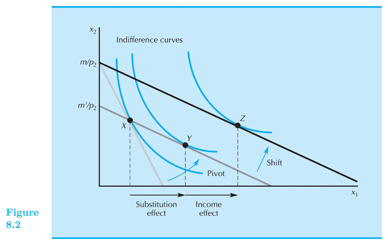

Inferior good: the income effect
is negative for one good
Giffen good: the income effect
is so negative that it outweighs the substitution effect and you buy less of a good when its price goes down!
Complements, Substitutes, Normal, and Inferior Goods
- Complements vs. Substitutes: relationship between X and Z
- Normal and Inferior Goods:
relationship between Y and Z
Next Time
- Cost minimization
- Relationship between utility and money
- Indirect utility functions
- Expenditure functions
Econ 50 | Spring 25 | Lecture 10
By Chris Makler
Econ 50 | Spring 25 | Lecture 10
Shifts in demand curves; offer curves; complements and substitutes; normal and inferior goods


