Profit Maximization
Christopher Makler
Stanford University Department of Economics
Econ 50 : Lecture 16
pollev.com/chrismakler

What color shirt am I wearing?
Today's Agenda
- Review of short-run costs
- Revenue as a function of \(q\)
- Profit as a function of \(q\)
- Everything this week is in the short run.
Theory of the Firm
Labor
Firm
🏭
Capital
⏳
⛏
Customers
🤓
p
w
r
q
L
K
Firms buy inputs
and produce some good,
which they sell to a customer.
PRICE
QUANTITY
Labor
w
L
Capital
r
K
Output
p
q
Firm
🏭
Costs
wL + rK
Revenue
pq
Theory of the Firm
Firms buy inputs
and produce some good,
which they sell to a customer.
PRICE
QUANTITY
Labor
w
L
Capital
r
K
Output
p
q
Costs
wL + rK
Revenue
pq
Profit
\pi = pq - (wL + rK)
Next week: Solve the optimization problem
finding the profit-maximizing quantity \(q^*\)
The difference between their revenue and their cost is what we call profits, denoted by the Greek letter \(\pi\).
Theory of the Firm
Costs
c(q) = wL(q) + rK(q)
Revenue
r(q) = p(q) \times q
Profit
\pi(q) = r(q) - c(q)
Theory of the Firm
Our approach will be to write costs, revenues, and profits all as functions of the ouput \(q\).
Profit
\pi(q) = r(q) - c(q)
Theory of the Firm
Our approach will be to write costs, revenues, and profits all as functions of the ouput \(q\).
We will then just take the derivative with respect to \(q\)
and set it equal to zero to find the firm's profit-maximizing quantity.
\pi'(q) = r'(q) - c'(q) = 0
r'(q) = c'(q)
MR
MC
Theory of the Firm
L^*(w,r,q)
K^*(w,r,q)
Exogenous Variables
Endogenous Variables
technology, \(f(L,K)\)
level of output, \(q\)
input prices \(w, r\)
Cost Minimization
Profit Maximization
cost function, \(c(w,r,q)\)
revenue function \(r(q)\)
\text{Optimal Output }q^*
Friday
Monday
Wednesday
Firm Production Functions and Cost Minimization
Profit Maximization
Input and Output Decisions of a Competitive Firm
Unit III: Theory of the Firm
Week 6
Week 7
Checkpoint II
Cost Functions
and Cost Curves
Elasticity and Market Power:
From Monopoly to Competition
Monday
Checkpoint III
Week 8
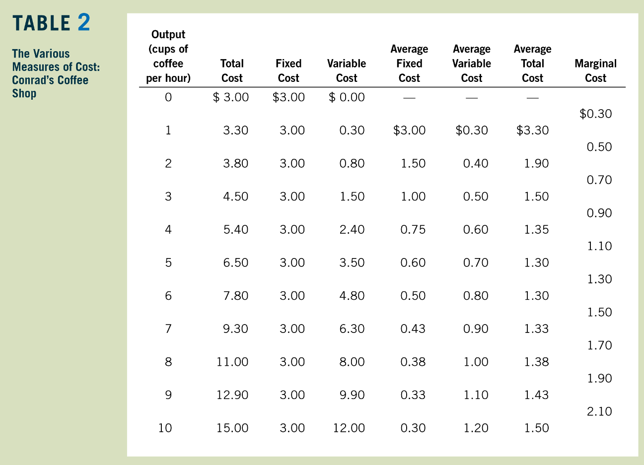
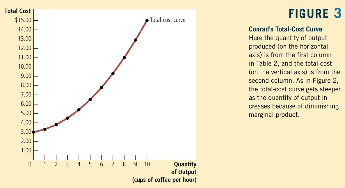
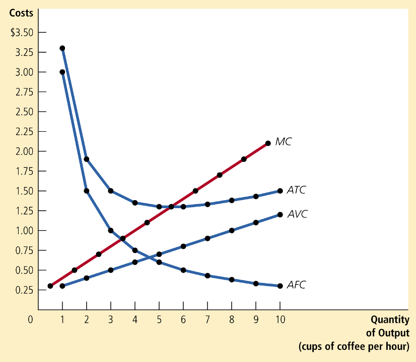
Review: Short-Run Costs
Greg Mankiw, Principles of Economics
Greg Mankiw, Principles of Economics
Dollars
Dollars Per Unit
Now assume that the level of capital is fixed in the short run at some amount \(\overline K\).
q = f(L\ |\ \overline K)
The amount of labor required to produce \(q\) units of output is therefore also going to depend upon \(\overline K\):
L(q\ |\ \overline K)
Short-Run Total Cost of \(q\) Units
TC(q\ |\ \overline{K}) = wL(q\ |\ \overline{K}) + r\overline{K}
Variable cost
"The total cost of producing \(q\) units in the short run is the variable cost of the required amount of the input that can be varied,
plus the fixed cost of the input that is fixed in the short run."
Fixed cost
f(L,K) = \sqrt{LK}
Short-run conditional demand for labor
if capital is fixed at \(\overline K\):
Total cost of producing \(q\) units of output:
L(q\ |\ \overline K) = {q^2 \over \overline K}
c(q\ |\ \overline{K}) = wL(q\ |\ \overline{K}) + r\overline{K} =
{wq^2 \over \overline K} + r\overline K
Example: \(w = 8\), \(r = 2\), \(\overline K =32\):
TC(q) = 64 + {1 \over 4}q^2
\text{Total Cost}: TC(q) = F + VC(q)
\text{Average Cost}: ATC(q) = \frac{TC(q)}{q} = \frac{F}{q} + \frac{VC(q)}{q}
Fixed Costs
Variable Costs
Average Fixed Costs (AFC)
Average Variable Costs (AVC)
Average Costs
\text{Total Cost}: TC(q) = F + VC(q)
\text{Average Cost}: ATC(q) = \frac{F}{q} + \frac{VC(q)}{q}
Average Costs
TC(q) = 64 + {1 \over 4}q^2
ATC(q) = {64 \over q} + {1 \over 4}q
\text{Total Cost}: TC(q) = F + VC(q)
\text{Marginal Cost}: MC(q) = TC'(q)
Marginal Cost
TC(q) = 64 + {1 \over 4}q^2
MC(q) = {1 \over 2}q
Relationship between Marginal Cost and Marginal Product of Labor
TC(q) = wL^c(q | \overline K) + r \overline K
{dTC(q) \over dq} = w \times {dL^c(q) \over dq}
= w \times {1 \over MP_L}
Revenue
Profit
The profit from \(q\) units of output
\pi(q) = r(q) - c(q)
PROFIT
REVENUE
COST
is the revenue from selling them
minus the cost of producing them.
Revenue
We will assume that the firm sells all units of the good for the same price, \(p\). (No "price discrimination")
r(q) = p(q) \times q
The revenue from \(q\) units of output
REVENUE
PRICE
QUANTITY
is the price at which each unit it sold
times the quantity (# of units sold).
The price the firm can charge may depend on the number of units it wants to sell: inverse demand \(p(q)\)
- Usually downward-sloping: to sell more output, they need to drop their price
- Special case: a price taker faces a horizontal inverse demand curve;
can sell as much output as they like at some constant price \(p(q) = p\)
Demand and Inverse Demand
Demand curve:
quantity as a function of price
Inverse demand curve:
price as a function of quantity
QUANTITY
PRICE
\text{revenue} = r(q) = p(q) \times q
\text{marginal revenue} = {dr \over dq} = {dp \over dq} \times q + p(q)
\displaystyle{\text{average revenue} = \frac{r(q)}{q} = p(q)}
If the firm wants to sell \(q\) units, it sells all units at the same price \(p(q)\)
Since all units are sold for \(p\), the average revenue per unit is just \(p\).
By the product rule...
let's delve into this...
Total, Average, and Marginal Revenue
\text{marginal revenue} = {dr \over dq} = {dp \over dq} \times q + p
dr = dp \times q + dq \times p
p
p(q)
q
The total revenue is the price times quantity (area of the rectangle)
\text{marginal revenue} = {dr \over dq} = {dp \over dq} \times q + p
dr = dp \times q + dq \times p
p
p(q)
q
dp
dq
The total revenue is the price times quantity (area of the rectangle)
If the firm wants to sell \(dq\) more units, it needs to drop its price by \(dp\)
Revenue loss from lower price on existing sales of \(q\): \(dp \times q\)
Revenue gain from additional sales at \(p\): \(dq \times p\)
Demand
Inverse Demand
q(p) = 20 - p
p(q) = 20-q
Revenue
r(q) =
MR(q)=
AR(q)=
20q - q^2
20 - 2q
20 - q
pollev.com/chrismakler
Suppose instead that the firm faced the demand function
(not inverse demand!)
\(q(p) = 20 - 2p\).
What would their marginal revenue function \(MR(q)\) be?
Correctness matters on this one...
Demand
Inverse Demand
q(p) = 20 - p
q(p) = 20 - 2p
p(q) = 20-q
p(q) = 10 - \tfrac{1}{2}q
Revenue
r(q) =
MR(q)=
AR(q)=
r(q) =
MR(q)=
AR(q)=
20q - q^2
20 - 2q
20 - q
10q - \tfrac{1}{2}q^2
10 - q
10 - \tfrac{1}{2}q
Profit
\pi(q) = \ \ \ \ \ \ \ \ \ \ \ \ \ \ \ \ \ \ -
Optimize by taking derivative and setting equal to zero:
\pi'(q) = \ \ \ \ \ \ \ \ \ \ \ \ \ \ \ \ - \ \ \ \ \ \ \ \ \ = 0
\Rightarrow \ \ \ \ \ \ \ \ \ \ \ \ \ \ =
Profit is total revenue minus total costs:
"Marginal revenue equals marginal cost"
(64 + {1 \over 4}q^2)
(20q - q^2)
r'(q)
c'(q)
{1 \over 2}q
20 - 2q
r'(q)
c'(q)
{1 \over 2}q
20 - 2q
40 - 4q = q
40 = 5q
q^* = 8
CHECK YOUR UNDERSTANDING
p(q)=20-2q
c(q)=10+5q+{1 \over 2}q^2
Find the profit-maximizing quantity.
Average Profit Analysis
\pi(q) = r(q) - c(q)
Multiply right-hand side by \(q/q\):
\pi(q) = \left[{r(q) \over q} - {c(q) \over q}\right] \times q
= (AR - AC) \times q
Profit is total revenue minus total costs:
"Profit per unit times number of units"
AVERAGE PROFIT
Next Time
- How does demand elasticity affect a firm's ability to mark up its price above marginal cost?
- Extreme example: a firm facing perfectly elastic demand (i.e., a "price taker" or "competitive firm")
Econ 50 | Fall 25 | Lecture 16
By Chris Makler
Econ 50 | Fall 25 | Lecture 16
Production and Cost for a Firm


