pollev.com/chrismakler

Will you need a left-handed desk for exams?
Demand Functions and Demand Curves
Christopher Makler
Stanford University Department of Economics
Econ 50: Lecture 8
where we'll be in week 7...
what we've done so far...
Friday
Monday
Wednesday
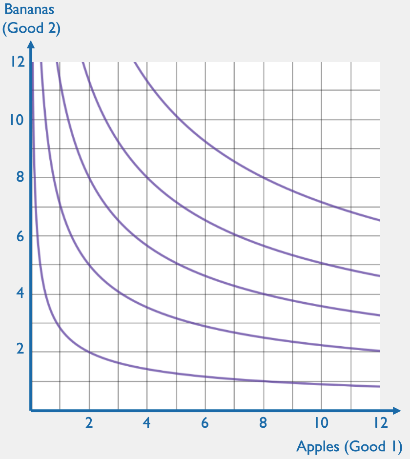
Preferences & Utility
Marginal Rate of Substitution
Utility Function Examples
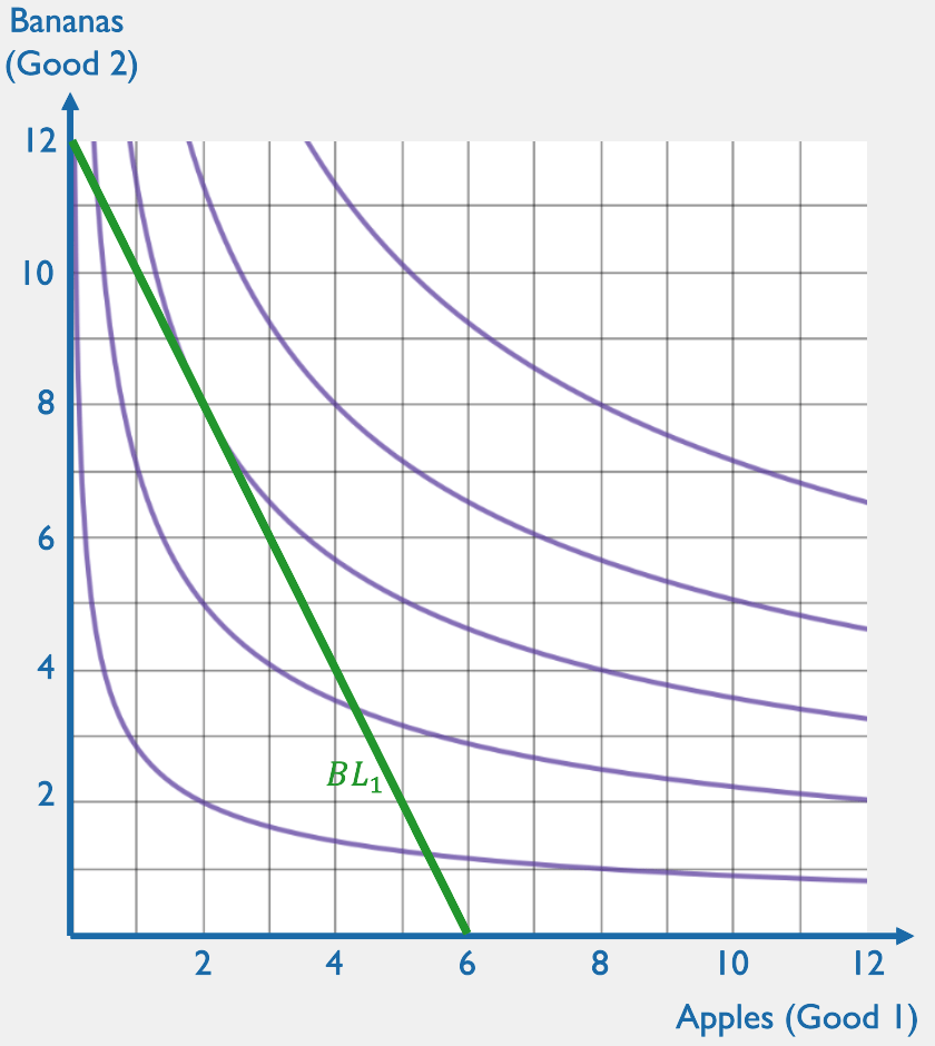
Budget Constraints
Utility Maximization subject to a Budget Constraint
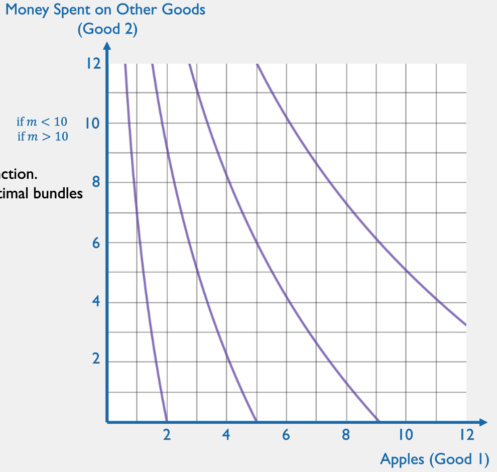
Cases when
Calculus Doesn't Work
Demand Functions and Demand Curves
Midterm I
Decomposing a Price Change into Income & Substitution Effects
Demand Curve Shifters: Complements & Substitutes
Unit I: Consumer Theory
Welcome
Week 1
Week 2
Week 3
Week 4
Cost Minimization
✅
✅
✅
✅
✅
✅
✅
IF...
THEN...
The consumer's preferences are "well behaved"
-- smooth, strictly convex, and strictly monotonic
\(MRS=0\) along the horizontal axis (\(x_2 = 0\))
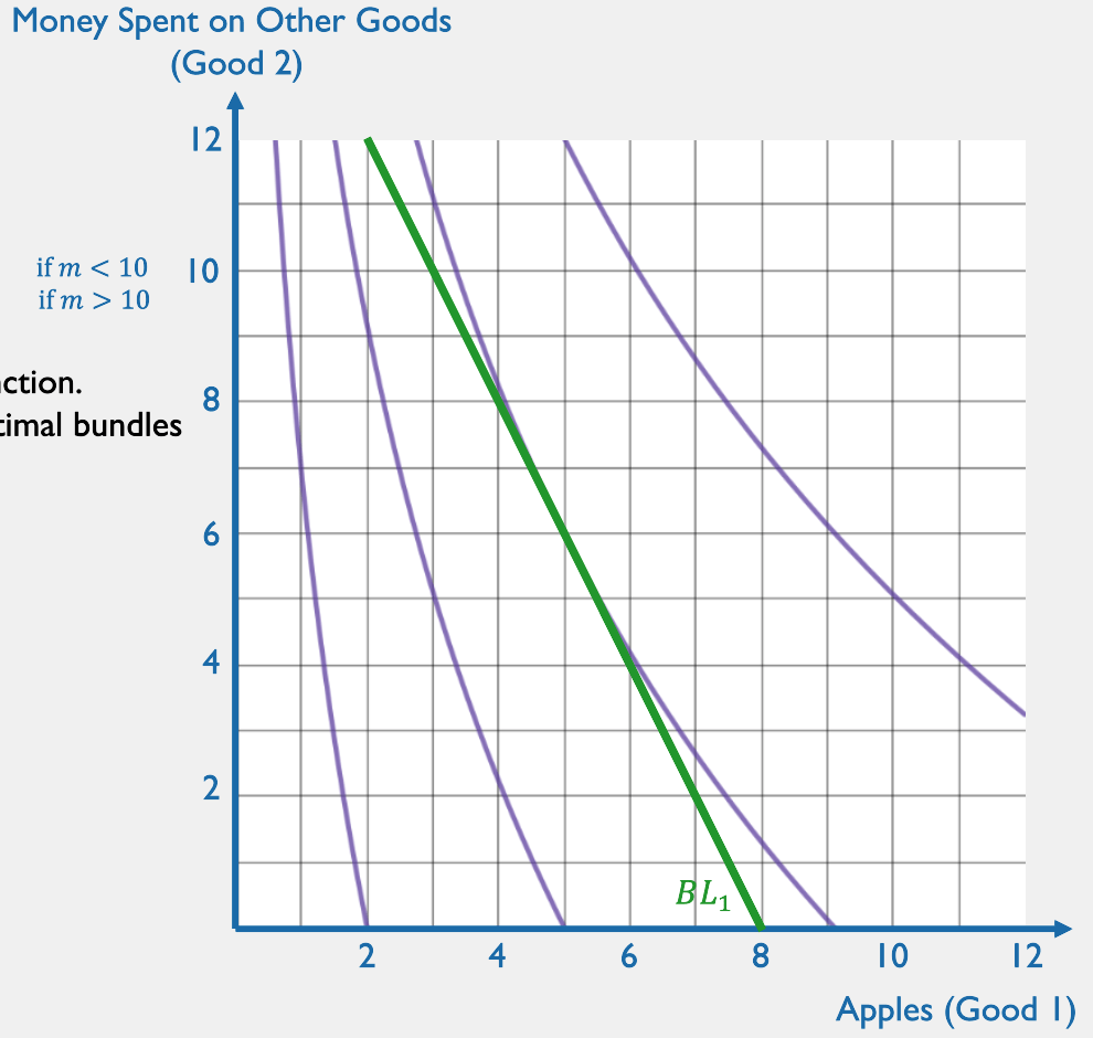
The budget line is a simple straight line
The optimal consumption bundle will be characterized by two equations:
MRS = \frac{p_1}{p_2}
p_1x_1 + p_2x_2 = m
More generally: the optimal bundle may be found using the Lagrange method
\(MRS \rightarrow \infty\) along the vertical axis (\(x_1 \rightarrow 0\))
Cobb-Douglas
Quasilinear
Perfect Substitutes
MRS = {ax_2 \over bx_1}
MRS = v'(x_1)
MRS = {a \over b}
u(x_1,x_2)=x_1^ax_2^b
u(x_1,x_2)=v(x_1) + x_2
u(x_1,x_2)=ax_1 + bx_2
TANGENCY CONDITION
x_2 = {p_1 \over p_2} \times {b \over a}x_1
v'(x_1) = {p_1 \over p_2}
{a \over b} = {p_1 \over p_2}
Ray from origin, will always intersect budget line =>
Lagrange always works
Vertical line, may or may not intersect BL in first quadrant =>
Lagrange sometimes works
Tries to equate two constants, which you just can't do =>
Lagrange never works
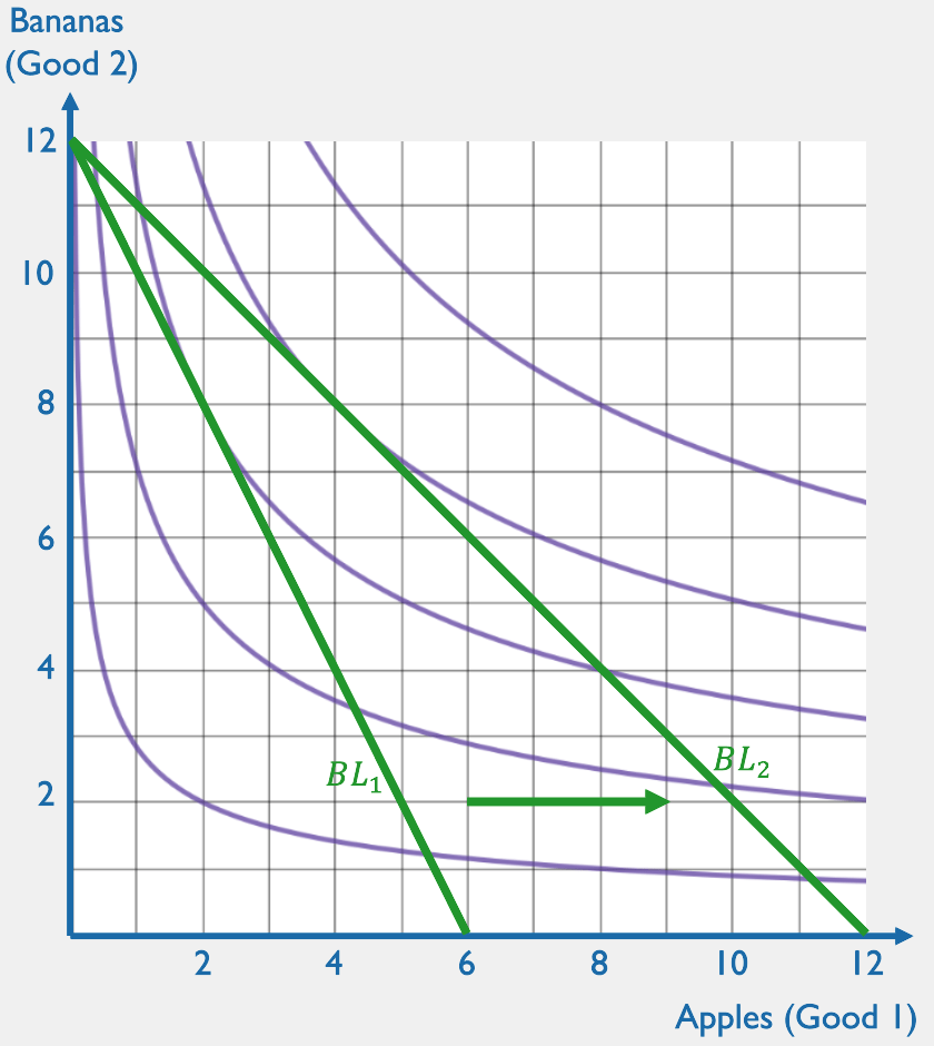
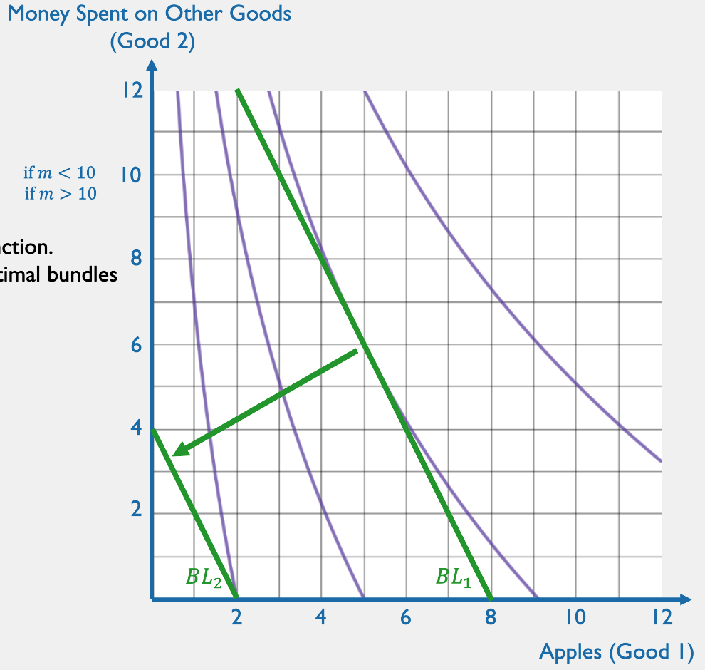
Last Class: What is the optimal bundle for a given budget line?
Today: What happens to the optimal bundle when prices/income change?
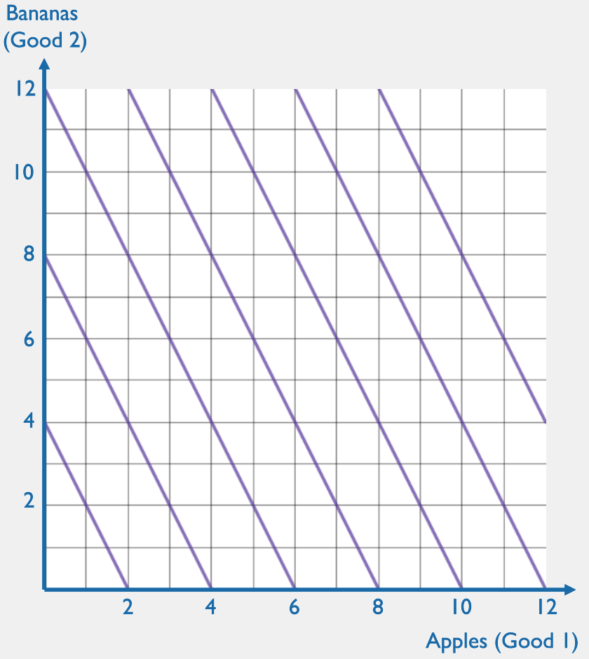
🍏
🍌
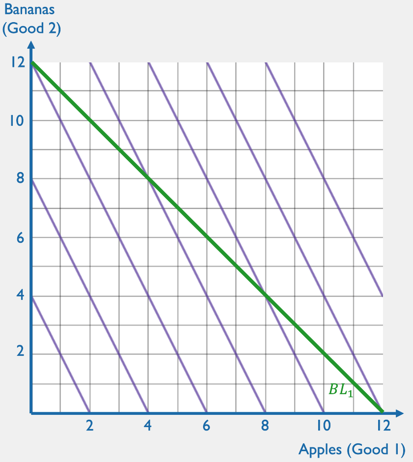
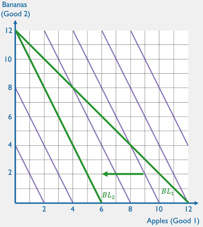
BL1
We will be solving for the optimal bundle
as a function of income and prices:
The solutions to this problem will be called the demand functions. We have to think about how the optimal bundle will change when \(p_1,p_2,m\) change.
x_1^*(p_1,p_2,m)
x_2^*(p_1,p_2,m)
BL2
Specific Prices & Income
General Prices & Income
\text{Constraint: }2 x_1 + x_2 = 12
Plug tangency condition back into constraint:
Tangency Condition: \(MRS = p_1/p_2\)
\text{Constraint: }p_1x_1 + p_2x_2 = m
\text{Objective function: } x_1^{1 \over 2}x_2^{1 \over 2}
MRS(x_1,x_2) = {x_2 \over x_1}
{x_2 \over x_1}
=
{2 \over 1}
\Rightarrow x_2 = 2x_1
{x_2 \over x_1}
=
{p_1 \over p_2}
\Rightarrow x_2 = {p_1 \over p_2}x_1
2x_1 + 2x_1 = 12
x_1^* = 3
p_1x_1 + p_2\left[{p_1 \over p_2}x_1\right] = m
x_1^*(p_1,p_2,m) = {m \over 2p_1}
4x_1 = 12
2p_1x_1 = m
x_2^* = 2x_1^* = 6
x_2^*(p_1,p_2,m) = {m \over 2p_2}
Specific Prices & Income
General Prices & Income
\text{Constraint: }2 x_1 + x_2 = 12
\text{Constraint: }p_1x_1 + p_2x_2 = m
\text{Objective function: } x_1^{1 \over 2}x_2^{1 \over 2}
MRS(x_1,x_2) = {x_2 \over x_1}
x_1^* = 3
x_1^*(p_1,p_2,m) = {m \over 2p_1}
x_2^* = 2x_1^* = 6
x_2^*(p_1,p_2,m) = {m \over 2p_2}
OPTIMAL BUNDLE
DEMAND FUNCTIONS
(optimization)
(comparative statics)
x_1^*(p_1,p_2,m)\ \
The Demand Function Illustrates Three Relationships
...its own price changes?
Movement along the demand curve
...the price of another good changes?
Complements
Substitutes
Independent Goods
How does the quantity demanded of a good change when...
...income changes?
Normal goods
Inferior goods
Giffen goods
(possible) shift of the demand curve
(Friday)
x_1^*(p_1,p_2,m)\ \
Three Relationships
...its own price changes?
Movement along the demand curve
How does the quantity demanded of a good change when...
The demand curve for a good
shows the quantity demanded of that good
as a function of its own price
holding all other factors constant
(ceteris paribus)
x_1
x_1
x_2
p_1
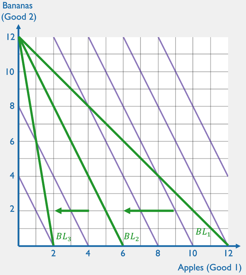
DEMAND CURVE FOR GOOD 1
BL_{p_1 = 2}
BL_{p_1 = 3}
BL_{p_1 = 4}
2
3
4
"Good 1 - Good 2 Space"
"Quantity-Price Space for Good 1"
BL
Note: Maximum Possible Quantity Demanded
\overline x_1 = {m \over p_1}


Quantity of Good 1 \((x_1)\)
Price of Good 1 \((p_1)\)
All demand curves must be in this region
Quantity bought at each price if you spent all your money on good 1
x_1 = {m \over p_1}
Cobb-Douglas Demand
Plug tangency condition into
the (generic) budget constraint:
Tangency Condition: \(MRS = p_1/p_2\)
u(x_1,x_2) = \ln x_1 + 2 \ln x_2
{x_2 \over 2x_1}
=
{p_1 \over p_2}
\Rightarrow x_2 = 2{p_1 \over p_2}x_1
p_1x_1 + p_2\left[2{p_1 \over p_2}x_1\right] = m
x_1^*(p_1,p_2,m) = {m \over 3p_1}
3p_1x_1 = m
Plug \(x_1^*(p_1,p_2,m)\) back
into the tangency condition:
x_2 = 2{p_1 \over p_2}\left[{m \over 3p_1}\right]
p_1x_1 + p_2x_2 = m
x_2 = 2{p_1 \over p_2}x_1
x_2^*(p_1,p_2,m) = {2m \over 3p_2}
Cobb-Douglas Demand
u(x_1,x_2) = \ln x_1 + 2 \ln x_2
x_1^*(p_1,p_2,m) = {m \over 3p_1}
x_2^*(p_1,p_2,m) = {2m \over 3p_2}
DEMAND FUNCTIONS
Let's think about how someone with preferences represented by this utility function would respond to a price change.
INITIAL BUDGET LINE
2x_1 + x_2 = 12
OPTIMAL BUNDLE
(2,8)
NEW BUDGET LINE
x_1 + x_2 = 12
OPTIMAL BUNDLE
(4,8)
Cobb-Douglas Demand
u(x_1,x_2) = \ln x_1 + 2 \ln x_2
x_1^*(p_1,p_2,m) = {m \over 3p_1}
x_2^*(p_1,p_2,m) = {2m \over 3p_2}
DEMAND FUNCTIONS
pollev.com/chrismakler
Q. What do these demand functions mean in words?
A. "Spend \({1 \over 3}\) of your income on good 1, and \({2 \over 3}\) of your income on good 2."
x_1^*(p_1,p_2,m) = \frac{a}{a+b}\times \frac{m}{p_1}
For a Cobb-Douglas utility function of the form
The “Cobb-Douglas Rule"
\text{(or equivalently) }u(x_1,x_2) = x_1^ax_2^b
The demand functions will be
x_2^*(p_1,p_2,m) = \frac{b}{a+b}\times \frac{m}{p_2}
That is, the consumer will spend fraction \(a/(a+b)\) of their income on good 1, and fraction \(b/(a+b)\) of their income on good 2.
This shortcut is very much worth memorizing! We'll use it a lot in the next few weeks in place of going through the whole optimization process.
u(x_1,x_2) = a \ln x_1 + b \ln x_2
Cobb-Douglas Demand
u(x_1,x_2) = \ln x_1 + 2 \ln x_2
x_1^*(p_1,p_2,m) = {m \over 3p_1}
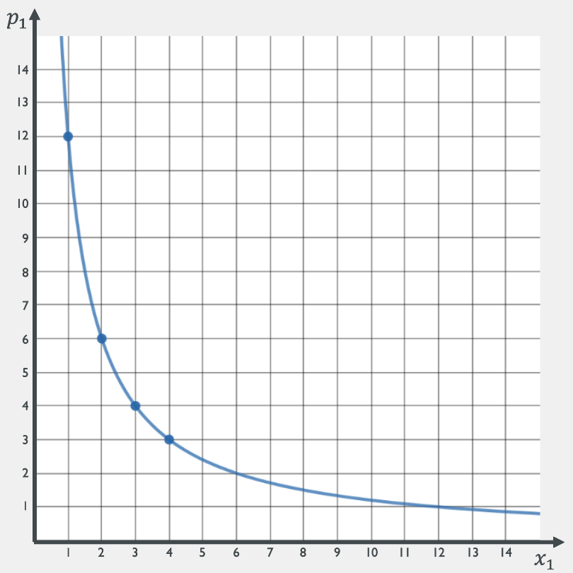
DEMAND FUNCTION FOR GOOD 1
DEMAND CURVE FOR GOOD 1
p_1
x_1(p_1,6,36)
Draw the demand curve if \(p_2 = 6\), \(m = 36\)
3
4
6
12
4
3
2
1
Cobb-Douglas Demand
u(x_1,x_2) = \ln x_1 + 2 \ln x_2
x_1^*(p_1,p_2,m) = {m \over 3p_1}
DEMAND FUNCTION FOR GOOD 1
DEMAND CURVE FOR GOOD 1
p_1
x_1(p_1,6,36)
Draw the demand curve if \(p_2 = 6\), \(m = 36\)
3
4
6
12
4
3
2
1
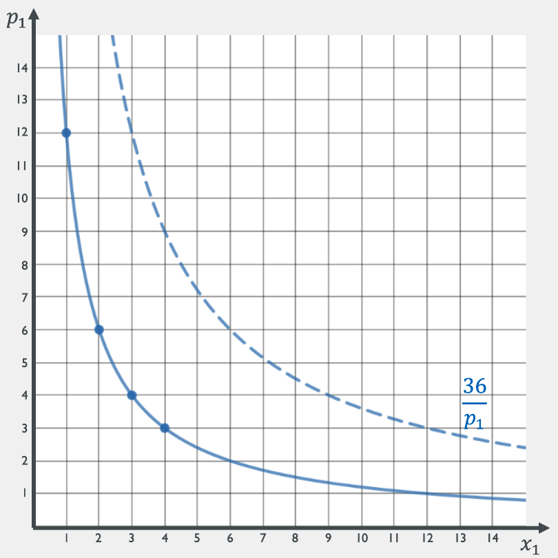
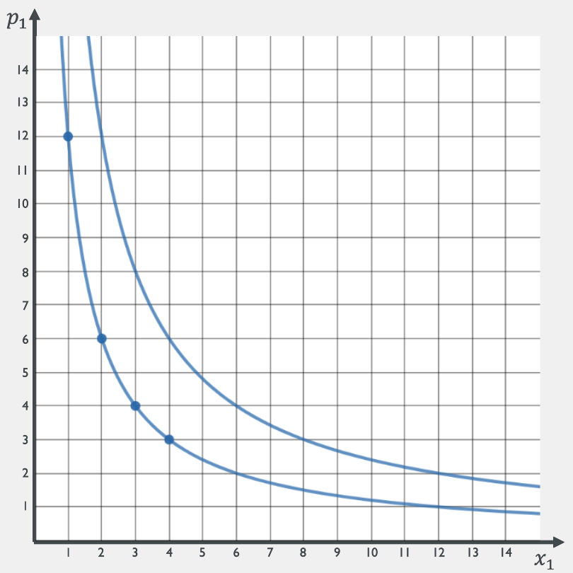
What happens if \(m\) increases to 72?
Cobb-Douglas Demand
u(x_1,x_2) = \ln x_1 + 2 \ln x_2
x_1^*(p_1,p_2,m) = {m \over 3p_1}
DEMAND FUNCTION FOR GOOD 1
DEMAND CURVE FOR GOOD 1
p_1
x_1(p_1,6,36)
Draw the demand curve if \(p_2 = 6\), \(m = 36\)
3
4
6
12
4
3
2
1
What happens if \(m\) increases to 72?
x_1(p_1,6,72)
8
6
4
2
Cobb-Douglas Demand Three Ways
x_1^*(p_1,p_2,m) = {m \over 3p_1}
x_2^*(p_1,p_2,m) = {2m \over 3p_2}
MATH
"Spend \({1 \over 3}\) of your income on good 1, regardless of prices and income."
GRAPHS
WORDS

Perfect Substitutes
When is the MRS greater than the price ratio? What would you buy in that case?
u(x_1,x_2) = 4x_1 + 2x_2
MRS = {MU_1 \over MU_2} = {4 \over 2} = 2
2 > {p_1 \over p_2}
p_1 < 2p_2
ONLY BUY GOOD 1
When is the MRS less than the price ratio? What would you buy in that case?
2 < {p_1 \over p_2}
p_1 > 2p_2
ONLY BUY GOOD 2
When is the MRS equal to the price ratio? What would you buy in that case?
2 = {p_1 \over p_2}
p_1 = 2p_2
BUY ANYTHING!
Perfect Substitutes
u(x_1,x_2) = 4x_1 + 2x_2
p_1 < 2p_2
ONLY BUY GOOD 1
p_1 > 2p_2
ONLY BUY GOOD 2
p_1 = 2p_2
BUY ANYTHING!
Consumer behavior:
MRS = {MU_1 \over MU_2} = {4 \over 2} = 2
Intuitive description of the behavior:
If you like apples twice as much as bananas,
you'll only buy apples as long as they cost less than twice as much as bananas do!
Perfect Substitutes: General Case
u(x_1,x_2) = ax_1 + bx_2
p_1 < {a \over b} p_2
ONLY BUY GOOD 1
p_1 > {a \over b}p_2
ONLY BUY GOOD 2
p_1 = {a \over b}p_2
BUY ANYTHING!
Consumer behavior:
How do we write this down as demand functions?
x_1^*(p_1,p_2,m)=
x_2^*(p_1,p_2,m)=
\begin{cases}
{m \over p_1} & \text{ if }p_1 < {a \over b}p_2\\ \\
\left[0, {m \over p_1}\right] & \text{ if }p_1 = {a \over b}p_2\\ \\
0 & \text{ if }p_1 > {a \over b}p_2
\end{cases}
\begin{cases}
{m \over p_2} & \text{ if }p_2 < {b \over a}p_1\\ \\
\left[0, {m \over p_2}\right] & \text{ if }p_2 = {b \over a}p_1\\ \\
0 & \text{ if }p_2 > {b \over a}p_1
\end{cases}
MRS = {MU_1 \over MU_2} = {a \over b}
Demand for Perfect Substitutes Three Ways
MATH
GRAPHS
WORDS
x_1^*(p_1,p_2,m)=
x_2^*(p_1,p_2,m)=
\begin{cases}
{m \over p_1} & \text{ if }p_1 < {a \over b}p_2\\ \\
\left[0, {m \over p_1}\right] & \text{ if }p_1 = {a \over b}p_2\\ \\
0 & \text{ if }p_1 > {a \over b}p_2
\end{cases}
\begin{cases}
{m \over p_2} & \text{ if }p_2 < {b \over a}p_1\\ \\
\left[0, {m \over p_2}\right] & \text{ if }p_2 = {b \over a}p_1\\ \\
0 & \text{ if }p_2 > {b \over a}p_1
\end{cases}
"Always buy whichever good gives you the higher bang for your buck"

Quasilinear
Plug tangency condition into
the (generic) budget constraint:
Tangency Condition: \(MU_1 = p_1\)
u(x_1,x_2) = 10\ln x_1 + x_2
{10 \over x_1}
=
{p_1}
\Rightarrow x_1 = {10 \over p_1}
p_1\left[{10 \over p_1}\right] + x_2 = m
x_2 = m - 10
p_1x_1 + x_2 = m
Suppose good 2 is "dollars spent on other goods," so \(p_2 = 1\).
Quasilinear
u(x_1,x_2) = 10\ln x_1 + x_2
x_1 = {10 \over p_1}
x_2 = m - 10
Suppose good 2 is "dollars spent on other goods," so \(p_2 = 1\).
Lagrange solutions:
Are these our demand functions?
BUDGET LINE
2x_1 + x_2 = 16
OPTIMAL BUNDLE
(5,6)
LAGRANGE SOLUTION
(5,6)
Quasilinear
u(x_1,x_2) = 10\ln x_1 + x_2
x_1 = {10 \over p_1}
x_2 = m - 10
Suppose good 2 is "dollars spent on other goods," so \(p_2 = 1\).
Lagrange solutions:
Are these our demand functions?
BUDGET LINE
2x_1 + x_2 = 4
OPTIMAL BUNDLE
(5,6)
LAGRANGE SOLUTION
(5,6)
Quasilinear
u(x_1,x_2) = 10\ln x_1 + x_2
x_1 = {10 \over p_1}
x_2 = m - 10
Suppose good 2 is "dollars spent on other goods," so \(p_2 = 1\).
Lagrange solutions:
Consumer behavior:
"If you have at least $10, spend $10 on apples. Otherwise, spend all your money on apples."
How do we write this down as demand functions?
x_1^*(p_1,m)=
x_2^*(p_1,m)=
\begin{cases}
{10 \over p_1} & \text{ if }m \ge 10\\ \\
{m \over p_1} & \text{ if }m \le 10
\end{cases}
\begin{cases}
{m - 10} & \text{ if }m \ge 10\\ \\
0 & \text{ if }m \le 10
\end{cases}
Demand with Quasilinear Preferences Three Ways
MATH
GRAPHS
WORDS
x_1^*(p_1,m)=
x_2^*(p_1,m)=
\begin{cases}
{10 \over p_1} & \text{ if }m \ge 10\\ \\
{m \over p_1} & \text{ if }m \le 10
\end{cases}
\begin{cases}
{m - 10} & \text{ if }m \ge 10\\ \\
0 & \text{ if }m \le 10
\end{cases}
"Buy up to the point where your MRS equal the price ratio, if you can afford it, regardless of your income."


This can feel like you're drinking from a fire hose.
You're not alone.
What we did today
- No new mathematical techniques!
- Solved for the optimal choice as a function of prices and income
- Plotted the demand curve for a good, holding the price of other goods and income constant.
- Section: some more drawing demand functions, plus looking over some old exam questions from HW
Econ 50 | Spring 25 | Lecture 8
By Chris Makler
Econ 50 | Spring 25 | Lecture 8
Demand Functions and Demand Curves


