Elasticity and Market Power:
From Monopoly to Competition
Christopher Makler
Stanford University Department of Economics
Econ 50: Lecture 17
Today's Agenda
- Overview of market structures
- Relationship between elasticity and marginal revenue
- Elasticity and profit maximization
- Special case: perfectly elastic demand and "competitive" (price-taking) firms
Part II: Implications for Profit Maximization
- Intuitive definition
- Mathematical definition
- Solving for elasticities using calculus
- Price elasticity of demand
Part I: Elasticity
Elasticity
Why Elasticity?

Notation
\epsilon_{Y,X} = \frac{\% \Delta Y}{\% \Delta X}
\text{Elasticity }(\epsilon) = \frac{\% \text{ change in endogenous variable}}{\% \text{ change in exogenous variable}}
"X elasticity of Y"
or "Elasticity of Y with respect to X"
Examples:
"Price elasticity of demand"
"Income elasticity of demand"
"Cross-price elasticity of demand"
"Price elasticity of supply"
Perfectly Inelastic
Inelastic
Unit Elastic
Elastic
Perfectly Elastic
|\epsilon| = 0
|\epsilon| < 1
|\epsilon| = 1
|\epsilon| > 1
|\epsilon| = \infty
Doesn't change
Changes by less than the change in X
Changes proportionally to the change in X
Changes by more than the change in X
Changes "infinitely" (usually: to/from zero)
How does the endogenous variable Y respond to a
change in the exogenous variable X?
\text{Elasticity }(\epsilon) = \frac{\% \text{ change in endogenous variable}}{\% \text{ change in exogenous variable}}
(note: all of these refer to the ratio of the perentage change, not absolute change)
Demand Elasticities
x_1^*(p_1,p_2,m)
How much of a good a consumer wants to buy, as a function of:
- the price of that good
- the price of other goods
- their income
We can ask: how much does the amount of this good change, when one of those determinants changes?
Price elasticity of demand: how the quantity demanded of a good changes due to a change in its own price.
\epsilon_{x_1,p_1} = \frac{\% \Delta x_1}{\% \Delta p_1}
pollev.com/chrismakler

If consumers respond to a 2% price increase by buying 3% less, demand at that price point is...?
Using Elasticities
- Suppose the price elasticity of demand is -2.
- This means that each % increase in the price
leads to approximately a 2% decrease in the quantity demanded - Example 1: a 3% increase in price would lead to a ~6% decrease in quantity
- Example 2: a 0.5% decrease in price would lead to a ~1% increase in quantity
- These are approximations in the same way as if \(dy/dx = -2\) along a function, increasing \(x\) by 3 would cause \(y\) to decrease by approximately 6.
\epsilon_{Y,X}
= \frac{\% \Delta Y}{\% \Delta X}
= \frac{\Delta Y / Y}{\Delta X / X}
= \frac{\Delta Y}{\Delta X}\times \frac{X}{Y}
\text{Suppose }Y \text{ is a function of }X.
General formula:
Linear relationship:
Using calculus:
Multiplicative relationship:
Y = mX + b
Y = f(X)
Y = aX^b
\text{General formula: }\epsilon_{Y,X} = \frac{\Delta Y}{\Delta X}\times \frac{X}{Y}
\text{If }Y = a + bX \text{, then }\frac{\Delta Y}{\Delta X} =
b
\epsilon_{Y,X} = b\times \frac{X}{a + bX}
Note: the slope of the relationship is \(b\).
Elasticity is related to, but not the same thing as, slope.
= \frac{bX}{a + bX}
\epsilon_{y,x}
= \frac{\% \Delta y}{\% \Delta x}
= \frac{\Delta y / y}{\Delta x / x}
= \frac{\Delta y}{\Delta x}\times \frac{x}{y}
\text{Suppose }y \text{ is a function of }x.
\text{In the limit, as }\Delta x \rightarrow 0:
\epsilon_{y,x} = \frac{dy}{dx}\times \frac{x}{y}
\text{General formula: }\epsilon_{y,x} = \frac{dy}{dx}\times \frac{x}{y}
\text{If }y = ax^b \text{, then }\frac{dy}{dx} =
abx^{b-1}
\epsilon_{y,x} = abx^{b-1} \times \frac{x}{ax^b}
= b
This is related to logs, in a way that you can explore in the homework.
This is a super useful trick and one that comes up on exams all the time!
Which part of a linear demand curve is more elastic?
Which part of a linear demand curve is more elastic?
Market Structures
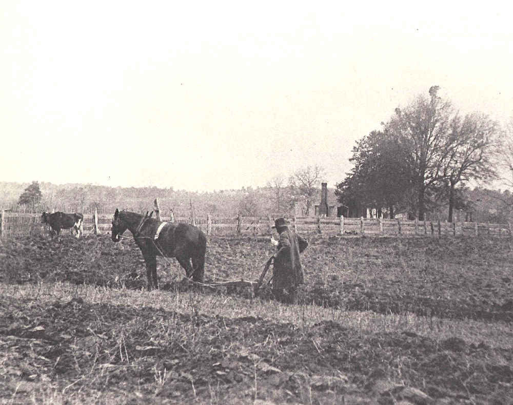
What were economists modeling when they came up with all these models?
Farmers producing commodities: price takers, no market power.
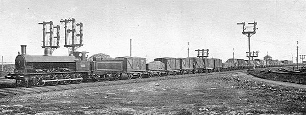
Railroads transporting goods:
price setters, lots of market power.
"Market Power" doesn't actually require a monopoly
Competition
- Lots of "small" firms selling basically the same thing
Market Power
- One or a few "medium" or "large" firms selling differentiated products
- Firms face essentially horizontal demand curve
- Firms face downward sloping demand curve
Monopoly as Metaphor
- True "monopolies" are rare
- Firms with some (at least local) market power are common
- We'll use "monopoly" as a metaphor
to analyze any firm that doesn't take prices as given,
and therefore faces a downward-sloping demand curve.
Revenue, Marginal Revenue, and Elasticity
\text{marginal revenue} = {dr \over dq} = {dp \over dq} \times q + p
dr = dp \times q + dq \times p
p
p(q)
q
The total revenue is the price times quantity (area of the rectangle)
\text{marginal revenue} = {dr \over dq} = {dp \over dq} \times q + p
dr = dp \times q + dq \times p
p
p(q)
q
dp
dq
Note: \(MR < 0\) if
dq \times p
{dq \over q} < {dp \over p}
\% \Delta q < \% \Delta p
|\epsilon| < 1
dp \times q
<
The total revenue is the price times quantity (area of the rectangle)
If the firm wants to sell \(dq\) more units, it needs to drop its price by \(dp\)
Revenue loss from lower price on existing sales of \(q\): \(dp \times q\)
Revenue gain from additional sales at \(p\): \(dq \times p\)
\text{marginal revenue} = {dr \over dq} = {dp \over dq} \times q + p
Marginal Revenue and Elasticity
= \left[{dp \over dq} \times {q \over p}\right] \times p + p
= \left[{1 \over \epsilon_{q,p}}\right] \times p + p
= p\left(1 - {1 \over |\epsilon_{q,p}|}\right)
(multiply first term by \(p/p\))
(definition of elasticity)
(since \(\epsilon < 0\))
Notes
Elastic demand: \(MR > 0\)
Inelastic demand: \(MR < 0\)
In general: the more elastic demand is, the less one needs to lower ones price to sell more goods, so the closer \(MR\) is to \(p\).
MR = p\left(1 - {1 \over |\epsilon_{q,p}|}\right)
The more elastic demand is, the less MR is different than price.
Profit Maximization and Elasticity
MR = p\left[1 - \frac{1}{|\epsilon_{q,p}|}\right]
We've just derived an elasticity
representation of marginal revenue:
MR = MC
Let's combine it with this
profit maximization condition:
p\left[1 - \frac{1}{|\epsilon_{q,p}|}\right] = MC
p = \frac{MC}{1 - \frac{1}{|\epsilon_{q,p}|}}
Really useful if MC and elasticity are both constant!
Inverse elasticity pricing rule:
p = \frac{MC}{1 - \frac{1}{|\epsilon_{q,p}|}}
If a firm has the cost function $$c(q) = 200 + 4q$$ and faces the demand curve $$D(p) = 6400p^{-2}$$ what is its optimal price?
Inverse elasticity pricing rule:
One more way of slicing it...
P = \frac{MC}{1 - \frac{1}{|\epsilon|}}
1 - \frac{1}{|\epsilon|} = \frac{MC}{P}
\frac{P - MC}{P} = \frac{1}{|\epsilon|}
Fraction of price that's markup over marginal cost
(Lerner Index)
What if \(|\epsilon| \rightarrow \infty\)?
Competitive (Price-Taking) Firms
Demand and Inverse Demand
Demand curve:
quantity as a function of price
Inverse demand curve:
price as a function of quantity
QUANTITY
PRICE
Special case: perfect substitutes
Demand and Inverse Demand
Demand curve:
quantity as a function of price
Inverse demand curve:
price as a function of quantity
QUANTITY
PRICE
Special case: perfect substitutes
For a small firm, it probably looks like this...
\text{marginal revenue} = {dr \over dq} = {dp \over dq} \times q + p
Marginal Revenue for Perfectly Elastic Demand
= \left[{dp \over dq} \times {q \over p}\right] \times p + p
= {p \over {dq \over dp} \times {p \over q}} + p
= p \left (1 - {1 \over |\epsilon_{q,p}|} \right)
(multiply first term by \(p/p\))
(simplify)
(since \(\epsilon < 0\))
Note
Perfectly elastic demand: \(MR = p\)
c(q) = 64 + {1 \over 4}q^2
r(q) = pq = 12q
\text{Let's assume }p = 12:
\text{Profit function is:}
\text{Total cost}
\pi(q) = 12q - [64 + {1 \over 4}q^2]
\text{Take derivative with respect to } q \text{ and set equal to zero:}
\pi'(q) = \ \ \ \ \ \ - \ \ \ \ \ \ = 0
12
{1 \over 2}q
Price
MC
\(q\)
$/unit
P = MR
12
MC = {1 \over 2}q
24
\Rightarrow q^* = 24
Summary
- All firms maximize profits by setting MR = MC
- If a firm faces a downward-sloping demand curve,
the marginal revenue is less than the price. - The more elastic a firm's demand curve,
the less it will optimally raise its price above marginal cost. - A competitive firm faces a perfectly elastic demand curve,
so its marginal revenue is equal to the price.
Econ 50 | Fall 25 | Lecture 17
By Chris Makler
Econ 50 | Fall 25 | Lecture 17
Profit Maximization, With and Without Market Power


