Book 1. Market Risk
FRM Part 2
MR 5. VaR Mapping
Presented by: Sudhanshu
Module 1. VaR Mapping
Module 2. Mapping Fixed-Income Securities
Module 3. Stress Testing, Perfomance Benchmarks and Mapping Derivatives
Module 1. VaR Mapping
Topic 1. Introduction to VaR Mapping
Topic 2. VaR Mapping Principles
Topic 3. VaR Mapping Process
Topic 4. Capturing General and Specific Risks using Mapping Process
Topic 5. Capturing General and Specific Risks using Mapping Process: Example
Topic 6. Computing General and Specific Risks using Mapping Process

Topic 1. Introduction to VaR Mapping
- Definition: Replacing portfolio positions with risk factor exposures to simplify risk management
- Process: Measure positions → map to risk factors using factor exposures → identify common factors across portfolio
- Purpose: Reduces variables when managing large portfolios with numerous positions
-
Benefits:
- Simplifies risk evaluation by consolidating positions into common factors (interest rates, equity prices, etc.)
- Handles securities with changing characteristics over time (e.g., fixed-income)
- Manages risk for assets lacking historical data (e.g., IPOs)
- Key advantage: Focuses on underlying risk factors rather than individual position prices when historical data is insufficient or irrelevant
Topic 2. VaR Mapping Principles
-
VaR Mapping Principles
- Aggregation: Combines risk exposures when analyzing each position individually is impractical due to excessive computations
- Simplification: Converts thousands of positions into primitive risk factors (e.g., one exchange rate factor for all related positions)
- Risk vs. Pricing: Aggregation acceptable for risk measurement even when prices cannot be aggregated for valuation purposes
- Time-based changes: Handles evolving exposures (e.g., bonds mapped to current spot yields as they mature; options as characteristics change)
- Data gaps: Provides solution when historical data is unavailable for positions
Topic 3. VaR Mapping Process
-
VaR Mapping Process
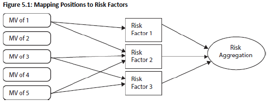
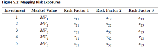
- Common factors identification: First step is identifying common risk factors, then matching market values of each position to those factors
- Risk factor distribution: Risk manager constructs distributions for identified risk factors and inputs data into the model
- Position allocation: Each position's market value (e.g., ) is allocated across its relevant risk factor exposures (e.g., )
- Systematic mapping: All portfolio positions are linked to their corresponding risk exposures in the same manner
- Aggregation: Column-wise summation of risk factors creates a vector of total risk exposures across the portfolio
Topic 4. Capturing General and Specific Risks using Mapping Process
-
General Risk Factors
-
Number of factors: In some cases, one or two general risk factors are sufficient to model a portfolio.
-
Trade-off: More risk factors = more time-consuming modeling BUT better approximation of portfolio risk exposure
-
Residual risk relationship: Number and type of risk factors directly affect magnitude of specific/unsystematic risk
-
-
Specific Risk
- Definition: Arises from asset-specific characteristics not captured by general risk factors
- Precision effect: More precisely defined risk factors → smaller residual/specific risk remaining
-
Example - bond portfolio:
- Duration only → large specific risk (ratings, terms, currencies unaccounted for)
- Add credit risk factor → reduced specific risk
- Add currency factor → further reduced specific risk
- Key principle: Specific risk is inversely related to comprehensiveness of general market risk factors chosen
Topic 5. Capturing General and Specific Risks using Mapping Process: Example
-
Problem scale: Portfolio of 5,000 stocks requires ~12.5 million covariance terms if each stock treated as separate risk factor ([5,000 × 4,999] / 2)
-
Risk decomposition: Each stock contains:
- Market risk component (systematic/beta risk)
- Firm-specific component (unsystematic risk)
- Diversification effect: Large portfolio diversifies away firm-specific components, leaving primarily market risk
- Mapping solution: Map market risk of all stocks onto single stock index factor (equity price changes)
- Result: Dramatically reduces parameters needed for risk calculation while capturing primary risk exposure
-
For an equity portfolio with N stocks mapped to a market index (primitive risk factor):
-
Risk Exposure (βi): Computed by regressing the return of stock 'i' on the market index return:
-
ϵi represents specific risk and is assumed to be uncorrelated with other stocks or the market portfolio.
-
-
Portfolio Return (Rp):
-
Aggregated Risk Exposure (βp):
-
Decomposition of Portfolio Return Variance, V(Rp):
-
General Market Risk:
-
Specific Risk:
-
Topic 6. Calculating General and Specific Risks using Mapping Process
Practice Questions: Q1
Q1. Which of the following could be considered a general risk factor?
I. Exchange rates.
II. Zero-coupon bonds.
A. I only.
B. II only.
C. Both I and II.
D. Neither I nor II.
Practice Questions: Q1 Answer
Explanation: A is correct.
Exchange rates can be used as general risk factors. Zero-coupon bonds are used to map bond positions but are not considered a risk factor. However, the interest rate on those zeros is a risk factor.
Module 2. Mapping Fixed-Income Securities
Topic 1. Mapping Portfolios of Fixed-Income Securities: Process
Topic 2. Mapping Portfolios of Fixed-Income Securities: Example
Topic 3. Principle Mapping
Topic 4. Duration Mapping
Topic 5. Cash Flow Mapping
Topic 1. Mapping Portfolios of Fixed-Income Securities: Process
-
Once general risk factors are selected, the portfolio is mapped onto these factors using one of three methods for fixed-income securities:
-
Principal Mapping: Considers only the risk of repayment of principal amounts.
-
Process: Uses the average maturity of the portfolio. VaR is calculated using the risk level from a zero-coupon bond that matches this average maturity.
-
Simplicity: It is the simplest of the three approaches.
-
-
Duration Mapping: The bond's risk is mapped to a zero-coupon bond with the same duration.
-
Process: VaR is calculated using the risk level of the zero-coupon bond that equals the portfolio's duration.
-
Challenge: It may be difficult to find a zero-coupon bond that exactly matches the portfolio's duration.
-
-
Cash Flow Mapping: The bond's risk is decomposed into the risk of each of its cash flows.
-
Precision: This is the most precise method because we map the present value of the cash flows (i.e., face amount discounted at the spot rate for a given maturity) onto the risk factors for zeros of the same maturities and include the inter-maturity correlations.
-
-
Practice Questions: Q1
Q1. Which of the following methods is not one of the three approaches for mapping a portfolio of fifixed-income securities onto risk factors?
A. Principal mapping.
B. Duration mapping.
C. Cash flow mapping.
D. Present value mapping.
Practice Questions: Q1 Answer
Explanation: D is correct.
Present value mapping is not one of the approaches
Topic 2. Mapping Portfolios of Fixed-Income Securities: Example
-
Let's illustrate the three mapping methods using a portfolio of two par value bonds:
-
Bond 1: One-year $100 million bond with a 3.5% coupon rate.
-
Bond 2: Five-year $100 million bond with a 5% coupon rate.
-
Total Portfolio Value: $200 million.
-
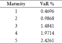
- VaR Percentages for Zero-Coupon Bonds (95% Confidence Level):
- The primary difference among these techniques lies in how they consider the timing and amount of cash flows.
Topic 3. Principle Mapping
-
Simplest Method: Only considers the timing of redemption or maturity payments, ignoring coupon payments.
-
Calculation:
-
Weights: Both bonds have a 50% weight ($100 million/$200 million).
-
Weighted Average Life of Portfolio: [0.50(1)+0.50(5)]=3 years.
-
Assumption: The entire portfolio value of $200 million occurs at the average life of three years.
-
VaR Percentage: For a three-year zero-coupon bond, the VaR percentage is 1.4841% (from table on previous slide).
-
Principal Mapping VaR: $200 million × 1.4841% = $2.968 million.
-
Practice Questions: Q2
Q2. If portfolio assets are perfectly correlated, portfolio VaR will equal:
A. marginal VaR.
B. component VaR.
C. undiversified VaR.
D. diversified VaR.
Practice Questions: Q2 Answer
Explanation: C is correct.
If we assume perfect correlation among assets, VaR would be equal to undiversified VaR.
Practice Questions: Q3
Q3. The VaR percentages at the 95% confidence level for a bond with maturities ranging from one year to five years are as follows:
A bond portfolio consists of a $100 million bond maturing in two years and a $100 million bond maturing in four years. What is the VaR of this bond portfolio using the principal VaR mapping method?
A. $1.484 million.
B. $1.974 million.
C. $2.769 million.
D. $2.968 million.
Practice Questions: Q3 Answer
Explanation: D is correct.
The VaR percentage is 1.4841 for a 3-year zero-coupon bond [(2 + 4)/2 =3]. We compute the VaR under the principal method by multiplying the VaR
percentage times the market value of the average life of the bond:
Principal mapping VaR = $200 million × 1.4841% = $2.968 million
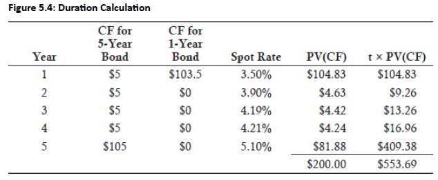
Topic 4. Duration Mapping
-
Concept: Replaces the portfolio with a ZCB having the same maturity as the portfolio's Macaulay duration.
-
Calculation (Macaulay Duration):
-
Numerator: Sum of (time × present value of cash flows)
-
Denominator: Present value of all cash flows.
-
Example: For the 2-bonds portfolio, Macaulay Duration = $553.69M/ $200M = 2.768 years.
-
-
Interpolating VaR:
-
VaR for a 2-year and 3-years ZCBs are 0.9868% and 1.4841% respectively
-
VaR for 2.768 years= 0.9868+(1.4841−0.9868)×(2.768−2)=0.9868+(0.4973×0.768)=1.3687%
-
-
Duration Mapping VaR= $200 million × 1.3687% = $2.737 million.
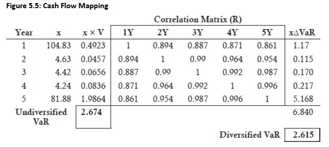
Topic 5. Cash Flow Mapping
-
Concept: Decomposes the bond's risk into the risk of each cash flow, mapping present values to ZCBs of the same maturities and including inter-maturity correlations (Fig 5.5).
-
Calculations:
-
First, present value of cash flows (PV(CF)) are determined.
-
Then, PV(CF) are multiplied by the corresponding zero-coupon VaR percentages.
-
Undiversified VaR: If all five ZCBs were perfectly correlated, the undiversified VaR is the sum of the absolute values of (present value of cash flows × VaR percentage).
-
For example, Undiversified VaR = 2.674 (sum of the 'x×V' column in Figure 5.5).
-
-
Diversified VaR: Requires incorporating the correlations between the ZCBs using a correlation matrix (R).
-
Computed using matrix algebra:
-
where 'x' is the present value of cash flows vector, 'V' is the vector of VaR for zero-coupon bond returns, and 'R' is the correlation matrix.
-
-
For the example, Diversified VaR (square root of 6.840) = 2.615.
-
-
Topic 5. Cash Flow Mapping
Module 3. Stress Testing, Perfomance Benchmarks and Mapping Derivatives
Topic 1. Stress Testing
Topic 2. Benchmarking a Portfolio
Topic 3. Benchmarking Process: Matching Duration with ZCBs
Topic 4. Benchmarking Process: Absolute VaR
Topic 5. Benchmarking Process: Tracking Error
Topic 6. Mapping Approaches for Linear Derivatives
Topic 7. Mapping Approach for Forward Contracts: Delta-Normal Method
Topic 8. Forward Contracts: Example Portfolio
Topic 9. Forward Contracts: Diversified and Undiversified VaR
Topic 10. Mapping Approach for Forward Rate Agreements (FRAs): Example Portfolio
Topic 11. Forward Rate Agreements (FRAs): Diversified and Undiversified VaR
Topic 12. Mapping Approach for Interest Rate Swaps
Topic 13. Mapping Approaches for Nonlinear Derivatives
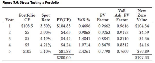
Topic 1. Stress Testing
-
Perfect Correlation Scenario: If perfect correlation is assumed among maturities of ZCBs, portfolio VaR equals undiversified VaR (sum of individual VaRs).
-
Stress Testing Approach: Instead of directly calculating undiversified VaR, each zero-coupon value can be reduced by its respective VaR, and the portfolio revalued. The difference between the revalued portfolio and the original portfolio value should equal the undiversified VaR.
-
Stressing each zero by its VaR is a simpler approach than incorporating correlations but is only viable if correlations are perfect (i.e., 1).
-
Example (Two-Bond Portfolio): Two-bond portfolio stress tested assuming perfectly correlated zeros; one-year zero-coupon bond has present value factor of 0.9662 at 3.5% discount rate
- VaR Calculation: At 95% confidence, the one-year bond has 0.4696% VaR movement, resulting in stressed value of 0.9616 [0.9662 × (1 − 0.4696/100)]
- Portfolio Impact: VaR-adjusted present values applied to cash flows yield portfolio value decline of $2.67 ($200.00 − $197.33), matching the undiversified VaR from the previous calculation
Topic 2. Benchmarking a Portfolio
-
Benchmarking a portfolio involves measuring VaR relative to a benchmark portfolio.
-
Portfolios can be constructed to match the risk factors of a benchmark but have a higher or lower VaR.
-
Tracking error VaR is the VaR of the deviation between the target portfolio and the benchmark portfolio. It measures the difference between the VaR of the target portfolio and the benchmark portfolio.
-
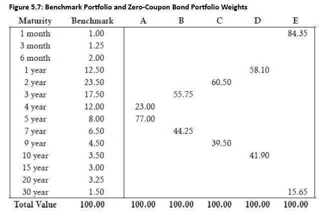
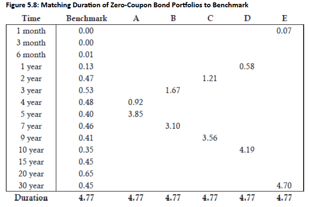
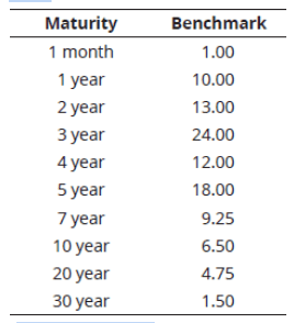
Example: Benchmark VaR of a $100 million bond portfolio (duration 4.77) against a two zero-coupon bond portfolio with matching duration at 95% confidence level
- Comparison Basis: Market value weights of bonds provided in Figure 5.7 for both the benchmark portfolio and the two zero-coupon bond portfolio
Topic 3. Benchmarking Process: Matching Duration with ZCBs
-
Consistent Approach: All other zero-coupon portfolios similarly adjust their two-bond weights to achieve the benchmark's target duration
-
Example - Portfolio A: Contains 4-year zero (23% weight) and 5-year zero (77% weight), yielding duration of 4.77, matching the benchmark
-
Five Portfolios Created: Figure 5.8 shows five two-bond portfolios, each with duration 4.77 achieved through different weight combinations
-
Duration Matching: Market value weights of zero-coupon bonds adjusted to match benchmark portfolio duration of 4.77
Topic 4. Benchmarking Process: Absolute VaR
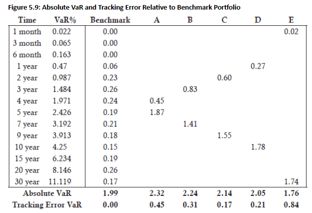
- Benchmark VaR Calculation: Absolute VaR computed by multiplying market value weights (Figure 5.7) by monthly VaR percentages (Figure 5.9), yielding $1.99 million—close to the 4-year note's VaR percentage
- Zero-Coupon Portfolio VaR: Absolute VaR for each of the five two-bond portfolios calculated by multiplying VaR percentage by market values of zero-coupon bonds
-
Tracking Error Setup: Relative performance measured as tracking error VaR, where x = market value positions of zero-coupon portfolios and x₀ = benchmark positions
-
Topic 5. Benchmarking Process: Tracking Error
- Tracking Error Source: Difference between benchmark and zero-bond portfolio VaR stems from nonparallel shifts in interest rate term structure
- Portfolio A Performance: Tracking error of $0.45 million is significantly lower than benchmark VaR of $1.99 million
- Portfolio C Optimal: Lowest tracking error at $0.17 million due to alignment with benchmark's largest weight in 2-year note (contains 2-year zero-coupon bond)
- VaR vs. Tracking Error: Minimizing absolute VaR differs from minimizing tracking error—Portfolio E (barbell structure) has lowest absolute VaR but highest tracking error to the index
-
Tracking error can be used to compute the variance reduction (similar to R-squared in a regression) as follows:
-
Variance improvement for Portfolio C relative to the benchmark is computed as:
Practice Questions: Q1
Q1. Suppose you are calculating the tracking error VaR for two zero-coupon bonds using a $100 million benchmark bond portfolio with the following maturities and market value weights. Which of the following combinations of two zero-coupon bonds would most likely have the smallest tracking error?
A. 1 year and 7 year.
B. 2 year and 4 year.
C. 3 year and 5 year.
D. 4 year and 7 year.
Practice Questions: Q1 Answer
Explanation: C is correct.
The three-year and five-year cash flows are highest for the benchmark portfolio at $24 million and $18 million, respectively. Thus, tracking error VaR will likely be the lowest for the portfolio where the cash flows of the benchmark and zero- coupon bond portfolios are most closely matched.
Topic 6. Mapping Approaches for Linear Derivatives
-
Delta-Normal Method: Provides accurate estimates of VaR for portfolios and assets that can be expressed as linear combinations of normally distributed risk factors.
-
Process: Once expressed as a linear combination of risk factors, a covariance (correlation) matrix can be generated, and VaR can be measured using matrix multiplication.
-
Applicability: This method is suitable for instruments like forwards, forward rate agreements, and interest rate swaps, as their values are linear combinations of a few general risk factors with readily available volatility and correlation data.
Topic 7. Mapping Approach for Forward Contracts: Delta-Normal Method
-
Current Value of a Forward Contract: Equal to the present value of the difference between the current forward rate (Ft) and the locked-in delivery rate (K):
-
Analogous Risk Positions: A forward position, such as purchasing euros with U.S. dollars, is analogous to three separate risk positions:
A short position in a U.S. Treasury bill.
A long position in a one-year euro bill.
A long position in the euro spot market.
Topic 8. Forward Contracts: Example Portfolio
-
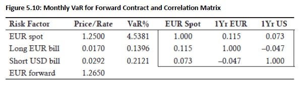
Example: Computing the diversified VaR of a forward contract used to purchase $100 million euros with $126.5 million U.S. dollars one year from now (pricing information in Fig 5.10).
-
Positions: A long position in a EUR contract worth $122.911 million today and a short position in a one-year U.S. T-bill worth $122.911 million today (shown in Fig 5.11).
-
Calculation Inputs: Requires pricing information for the forward contract and the correlation matrix between the positions. The absolute present value of cash flows is multiplied by the VaR percentage.
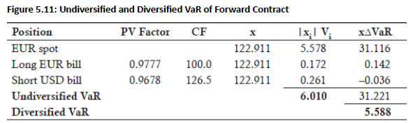
Topic 9. Forward Contracts: Diversified and Undiversified VaR
-
Undiversified VaR: For the forward contract example, the undiversified VaR is $6.01 million. This is computed as the sum of the absolute present values of cash flows multiplied by their respective VaR percentages.
-
Diversified VaR: For the forward contract example, the diversified VaR is $5.588 million. This is computed using matrix algebra, multiplying the vector of absolute values by the correlation matrix.
Topic 10. Mapping Approach for Forward Rate Agreements (FRAs): Example Portfolio
-
Concept: The general procedure for forwards also applies to FRAs.
-
Example: Selling a 6x12 FRA on $100 million (data shown in Fig 5.12). This is equivalent to borrowing $100 million for 6 months (180 days) and investing at the 12-month rate (360 days).
-
Present Values of Cash Flows: If the 360-day spot rate is 4.5% and the 180-day spot rate is 4.1%, the present value of the notional $100 million contract is x = $100 / 1.0205 = $97.991 million.
-
Forward Rate: Computed as (1+F1,2/2)=[1.045/(1+0.041/2)]=[(1.045/1.0205)−1]×2=4.8%
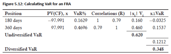
Topic 11. Forward Rate Agreements (FRAs): Diversified and Undiversified VaR
-
Undiversified VaR: Computed by multiplying the VaR percentages by the absolute value of the present values of cash flows and summing them. For the FRA example, the undiversified VaR is $0.62 million at the 95% confidence level.
-
Diversified VaR: Matrix algebra is used to multiply the vector (from the undiversified VaR calculation) by the correlation matrix. For the FRA example, the diversified VaR is $0.348 million.
Topic 12. Mapping Approach for Interest Rate Swaps
-
Decomposition: Interest rate swaps can be broken down into fixed and floating parts.
-
The fixed part is priced with a coupon-paying bond.
-
The floating part is priced as a floating-rate note.
-
-
VaR Calculation Steps (Undiversified and Diversified):
-
Create Present Value of Cash Flows: Show a short position for the fixed portion (paying fixed interest rates and fixed bond maturity) and a long present value for the variable rate bond.
-
Compute Undiversified VaR: Multiply the vector representing the absolute present values of cash flows by the VaR percentages (e.g., at 95% confidence) and sum the values.
-
Compute Diversified VaR: Use matrix algebra to multiply the correlation matrix by the absolute values.
-
Topic 13. Mapping Approaches for Nonlinear Derivatives
-
Challenge: The delta-normal VaR method relies on linear relationships between variables. Options, however, exhibit nonlinear relationships between movements in the underlying instrument's value and the option's value.
-
Applicability: In many cases, the delta-normal method can still be applied because an option's value can be expressed linearly as the product of the option's delta.
-
Limitations: Delta-normal VaR may not provide accurate VaR measures over long risk horizons where deltas are unstable.
-
Options are usually mapped using a Taylor series approximation and using the delta-gamma method to calculate the option VaR.