El criterio de estabilidad de Lyapunov
IE3041 - Sistemas de Control 2

El concepto más importante en sistemas de control
cualidad interna de sistemas dinámicos
evolución a largo plazo sin resolver la ED
estrechamente relacionada al control
cualidad interna de sistemas dinámicos
evolución a largo plazo sin resolver la ED
estrechamente relacionada al control
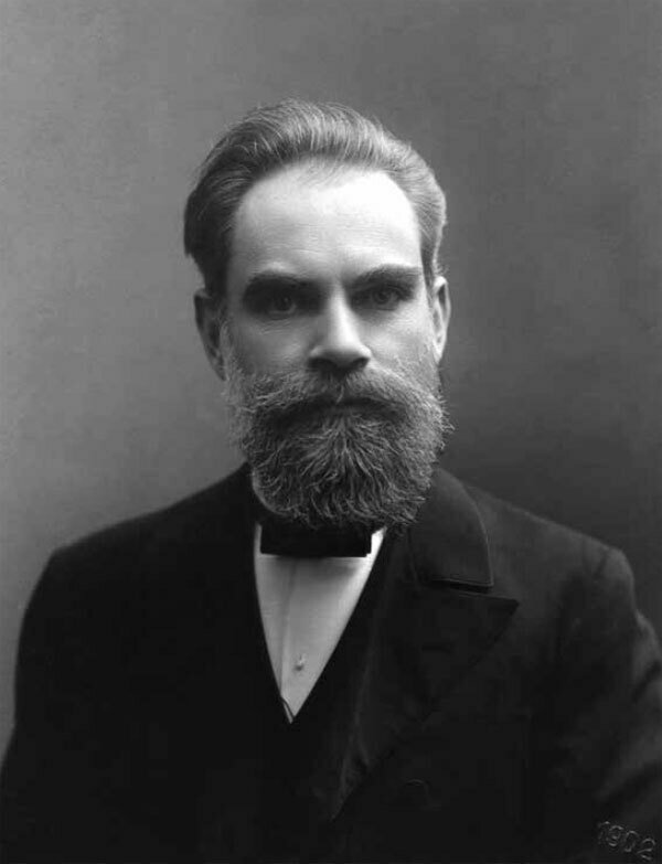
Aleksandr Lyapunov
Conjuntos invariantes y límite
sistemas no lineales
Conjuntos invariantes y límite
sistemas no lineales
diversos comportamientos en el espacio de estados
Conjuntos invariantes y límite
sistemas no lineales
diversos comportamientos en el espacio de estados
NO existe una noción global de estabilidad
Conjuntos invariantes y límite
sistemas no lineales
diversos comportamientos en el espacio de estados
NO existe una noción global de estabilidad
(sólo local)
Conjuntos invariantes y límite
sistemas no lineales
diversos comportamientos en el espacio de estados
NO existe una noción global de estabilidad
(sólo local)
"estabilidad de comportamientos"
requiere definir conjuntos especiales
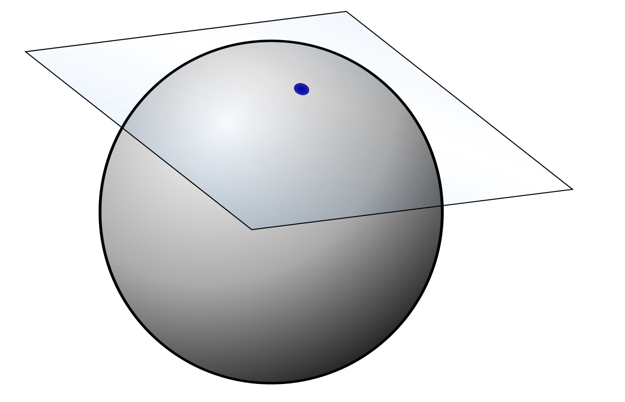
Conjunto invariante positivo
Conjunto invariante positivo
Conjunto invariante positivo
Conjunto límite\(-\omega\)
Conjunto límite\(-\omega\)
Conjunto límite\(-\omega\)
Conjunto límite\(-\omega\)
distancia hacia el conjunto
puede ser en tiempo finito
Conjunto límite\(-\omega\)
distancia hacia el conjunto
puede ser en tiempo finito
conjunto invariante positivo atractor
Conjunto límite\(-\alpha\)
Conjunto límite\(-\alpha\)
Conjunto límite\(-\alpha\)
Conjunto límite\(-\alpha\)
Conjunto límite\(-\alpha\)
conjunto repulsor
Algunos ejemplos de conjuntos de interés
Órbita periódica
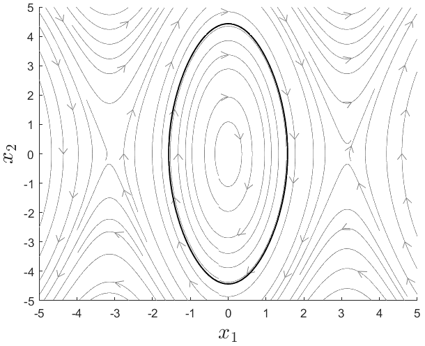
Ej. péndulo simple
ie3041_clase4_periodic_orbitÓrbita periódica
Ej. péndulo simple
conjunto invariante positivo
ie3041_clase4_periodic_orbitCiclo límite
ie3041_clase4_limit_cycle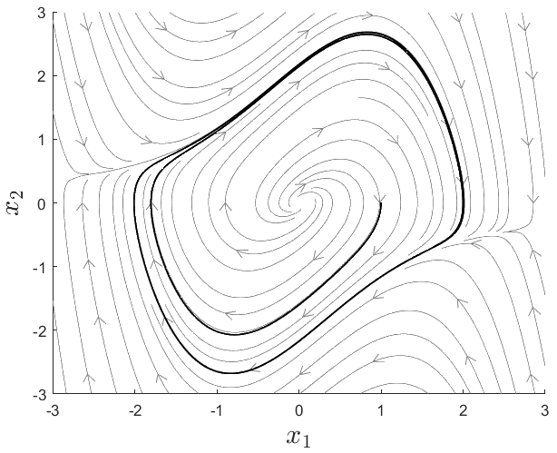
Ej. oscilador de Van der Pol
Ciclo límite
Ej. oscilador de Van der Pol
conjunto límite\(-\omega\) (atractor, asumiendo \(t>0\))
ie3041_clase4_limit_cycleórbita periódica atractora
Ciclo límite
Ej. oscilador de Van der Pol
conjunto límite\(-\omega\) (atractor, asumiendo \(t>0\))
ie3041_clase4_limit_cycleórbita periódica atractora
también existen ciclos límite repulsores, aunque no son tan comunes
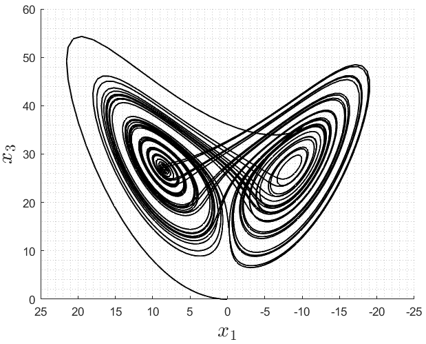
Atractor extraño
Ej. sistema de Lorenz
conjunto límite\(-\omega\)
(con estructura fractal)
ie3041_clase4_strange_attractorsistemas caóticos
Puntos fijos o de equilibrio
Ej. sistema LTI 1
ie3041_clase4_fixed_point1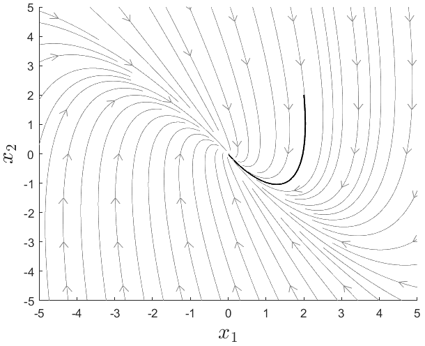
Puntos fijos o de equilibrio
Ej. sistema LTI 1
conjunto límite\(-\omega\)
(atractor)
ie3041_clase4_fixed_point1Puntos fijos o de equilibrio
Ej. sistema LTI 2
ie3041_clase4_fixed_point2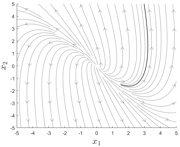
Puntos fijos o de equilibrio
Ej. sistema LTI 2
conjunto límite\(-\alpha\)
(repulsor)
ie3041_clase4_fixed_point2Puntos fijos o de equilibrio
Ej. sistema LTI 2
conjunto límite\(-\alpha\)
(repulsor)
ie3041_clase4_fixed_point2el criterio de estabilidad se planteó originalmente para puntos de equilibrio
Estabilidad en el sentido de Lyapunov
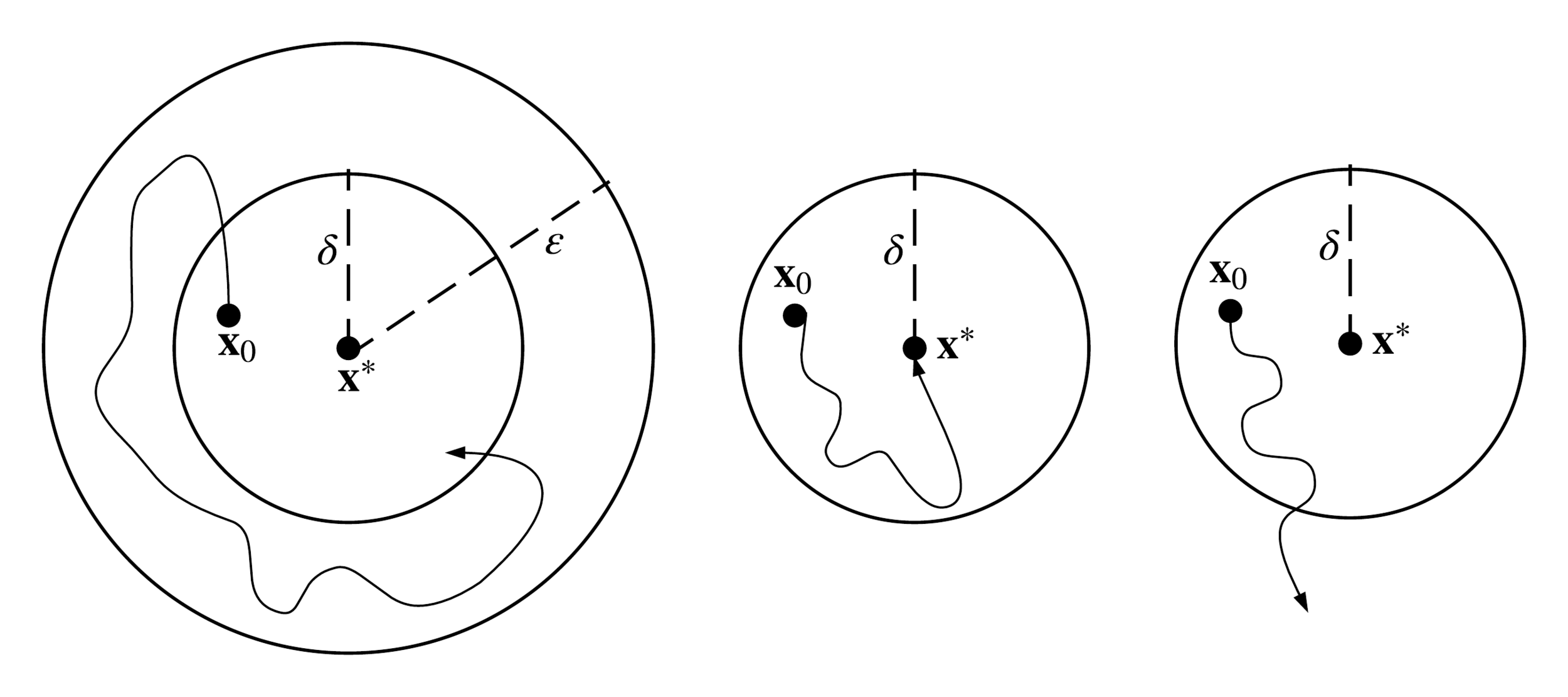
(localmente) estable
(localmente) asintóticamente estable (A.S.)
inestable
si NO es estable
exponencialmente estable
(caso especial de A.S.)
Caso especial: sistemas LTI
Caso especial: sistemas LTI
Caso especial: sistemas LTI
\(\mathbf{x}^*=\mathbf{0}\) único punto de equilibrio*
*excluyendo al espacio nulo de \(\mathbf{A}\)
por lo tanto, toda condición de estabilidad es global para sistemas LTI
por lo tanto, toda condición de estabilidad es global para sistemas LTI
estabilidad del sistema LTI \(\Leftrightarrow\) estabilidad del punto \(\mathbf{x}^*=\mathbf{0}\)
por lo tanto, toda condición de estabilidad es global para sistemas LTI
estabilidad del sistema LTI \(\Leftrightarrow\) estabilidad del punto \(\mathbf{x}^*=\mathbf{0}\)
SIN EXCEPCIONES
la estabilidad de \(\mathbf{x}^*=\mathbf{0}\) depende únicamente de \(\sigma\left(\mathbf{A}\right)\equiv\) los eigenvalores de \(\mathbf{A}\)
la estabilidad de \(\mathbf{x}^*=\mathbf{0}\) depende únicamente de \(\sigma\left(\mathbf{A}\right)\equiv\) los eigenvalores de \(\mathbf{A}\)
¿Por qué?
la estabilidad de \(\mathbf{x}^*=\mathbf{0}\) depende únicamente de \(\sigma\left(\mathbf{A}\right)\equiv\) los eigenvalores de \(\mathbf{A}\)
¿Por qué?
polos = eig(A)la estabilidad de \(\mathbf{x}^*=\mathbf{0}\) depende únicamente de \(\sigma\left(\mathbf{A}\right)\equiv\) los eigenvalores de \(\mathbf{A}\)
¿Por qué?
polos = eig(A)luego de lo cual aplican los mismos* criterios que en control clásico
mismos*, aunque podemos ser más específicos:
el caso de asintóticamente estable se promueve a Globalmente Exponencialmente Asintóticamente Estable (G.A.S.)
mismos*, aunque podemos ser más específicos:
marginalmente/críticamente estable requiere que los polos con \(\mathrm{Re}(\lambda)=0\) tengan multiplicidad algebráica unitaria
para este caso también \(\displaystyle\lim_{t\to\infty} \mathbf{x}(t) \in \mathcal{N}\left(\mathbf{A}\right)\)
Estabilidad BIBO
sistema de control BIBO (Bounded-Input Bounded-Output) estable si
Estabilidad BIBO
sistema de control BIBO (Bounded-Input Bounded-Output) estable si
sistema LTI G.A.S. \(\Leftrightarrow\) sistema LTI BIBO estable*
*casi siempre
¿Estabilidad en sistemas no lineales?
¿Estabilidad en sistemas no lineales?
diversos comportamientos
\(\Rightarrow\) "diversas estabilidades"
¿Estabilidad en sistemas no lineales?
diversos comportamientos
\(\Rightarrow\) "diversas estabilidades"
Idea
empleemos sistemas LTI para "capturar las estabilidades"
¿Estabilidad en sistemas no lineales?
diversos comportamientos
\(\Rightarrow\) "diversas estabilidades"
Idea
empleemos sistemas LTI para "capturar las estabilidades"
esto se conoce como el método indirecto de Lyapunov
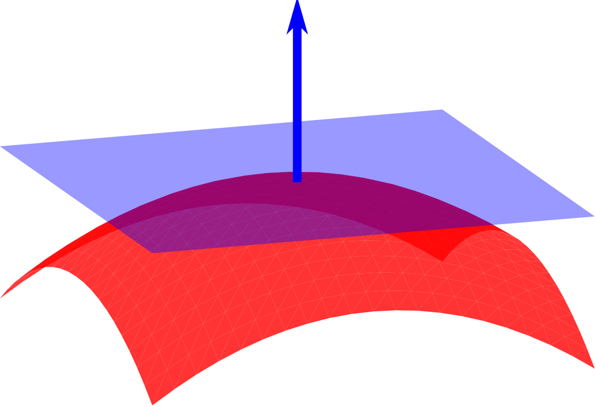
El teorema de Hartman-Grobman
"El comportamiento local de un sistema dinámico no lineal alrededor de un punto de equilibrio hiperbólico, es cualitativamente el mismo que el de su linealización alrededor de dicho punto de equilibrio."
El teorema de Hartman-Grobman
"El comportamiento local de un sistema dinámico no lineal alrededor de un punto de equilibrio hiperbólico, es cualitativamente el mismo que el de su linealización alrededor de dicho punto de equilibrio."
El método indirecto de Lyapunov
El método indirecto de Lyapunov
El método indirecto de Lyapunov
linealización
El método indirecto de Lyapunov
linealización
G.A.S
A.S
El método indirecto de Lyapunov
linealización
G.A.S
A.S
inestable
inestable
El método indirecto de Lyapunov
linealización
G.A.S
A.S
inestable
inestable
punto hiperbólico
El método indirecto de Lyapunov
linealización
marginalmente estable
G.A.S
A.S
inestable
inestable
???
punto hiperbólico
Ejemplo: estabilidad péndulo invertido
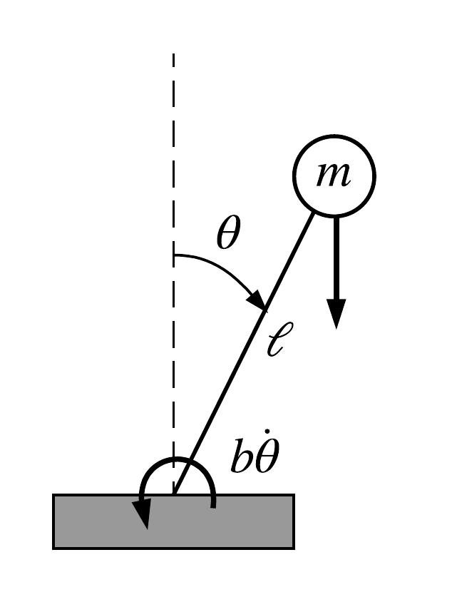
Ejemplo: estabilidad péndulo invertido
(localmente) inestable
localmente A.S.
>> ie3041_clase4_invpend.mlx