Production and Cost
for a Firm
Christopher Makler
Stanford University Department of Economics
Econ 50 : Lecture 13
pollev.com/chrismakler

How did the midterm go, relative to how you expected it to go?
So, about that test...
Remember that the purpose of this test was primary feedback:
reveal to yourselves where your understanding is squishy.
Key insight: you will only buy the good with the highest "boom for the buck" (i.e., \(MU/p\)).
What does this tell us about goods 2 and 3?
You will never buy good 2!
Key insight: you will only buy the good with the highest "boom for the buck" (i.e., \(MU/p\)).
When will you only buy good 1?
Key insight: you will only buy the good with the highest "boom for the buck" (i.e., \(MU/p\)).
When will you only buy good 1?
Key insight: you will only buy the good with the highest "boom for the buck" (i.e., \(MU/p\)).
What happens if you try to equate the MU/p across goods (or equivalently, set the MRS's equal to the price ratios)?

About 48% of students approached that question
the correct way.
You are not alone.
Remember: the lower of your two midterm scores only counts for 10% of your grade.
If you get a 50 on the midterm (curved), you can still get as high as a 95% in the class.
But: if you struggled a lot on the test,
it means you should do something different about how you approach the class
The fact that so many of you strugged with a basic intuitive concept also means that I need to do something different about how I approach the class.


How class participation will count toward your grade
- I will use PollEv to keep track of who has attended each lecture
- If you do badly on an exam question, I will look to see if you missed class on the day related to that question.
- If you were in class or had an excused absence*, I will add a few points back. If you just skipped class that day, I will have less sympathy.
- So: you can still get 100% if you never come to class and ace all the exams; but if you do badly on an exam, showing that you were in class can help mitigate the damage.
- *You may not have too many excused absences. (You can't just call in sick for the rest of the term.)
Today's Agenda
- Review of Econ 1 Treatment of Production and Cost
- Total, Average, and Marginal Costs
- Long-Run Costs and Returns to Scale
- Short-Run Costs and the Marginal Product of Labor
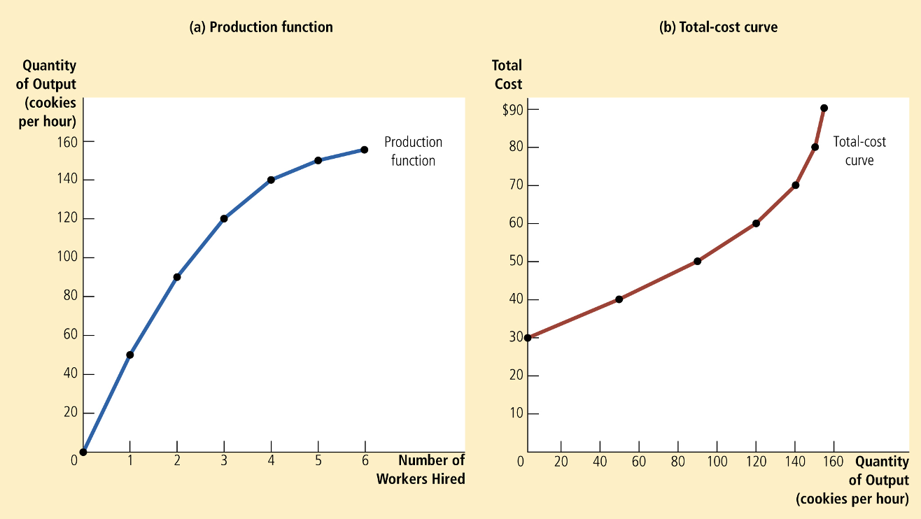
The Econ 1 Approach
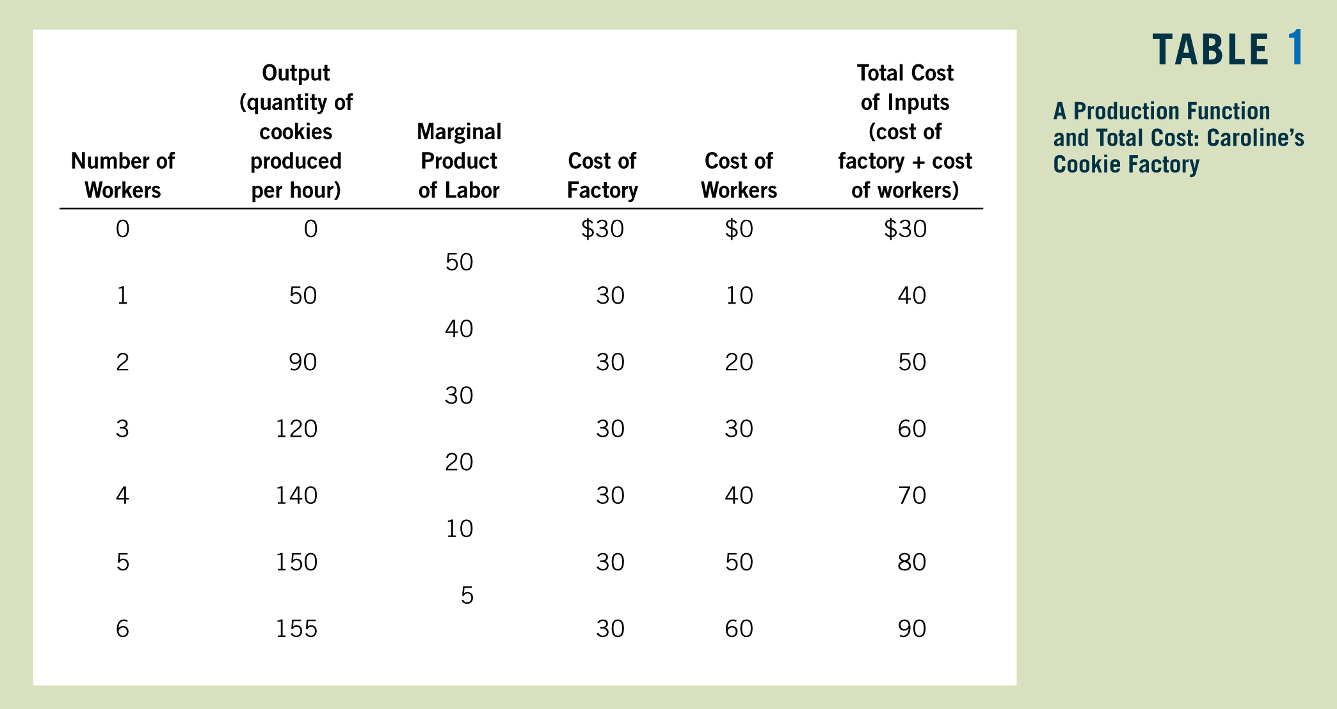
Greg Mankiw, Principles of Economics
Greg Mankiw, Principles of Economics
Greg Mankiw, Principles of Economics
Greg Mankiw, Principles of Economics
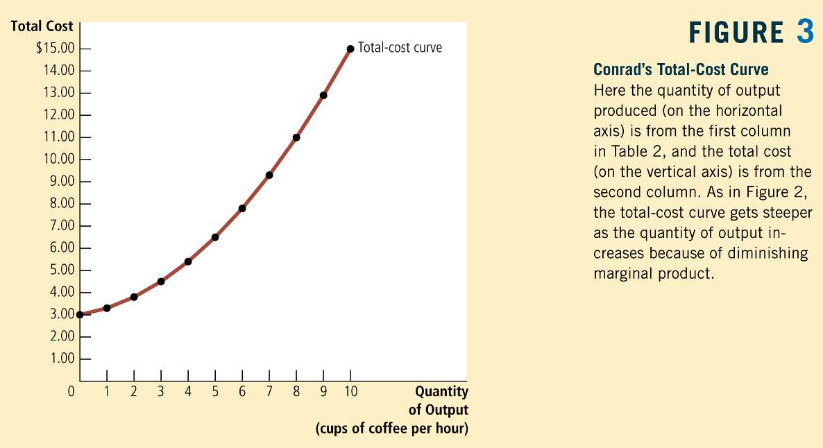
Greg Mankiw, Principles of Economics
Dollars
Dollars Per Unit
Greg Mankiw, Principles of Economics

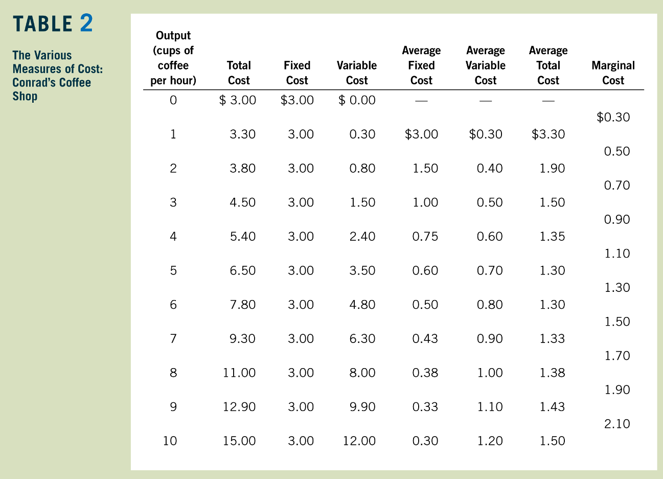
Total, Average, and Marginal Costs
Total Cost:
Average Cost:
Marginal Cost:

Suppose it costs $100,000 to fly 200 passengers from SFO to NYC
Marginal cost tends to "pull" average cost toward it:
Marginal grade = grade on last test, average grade = GPA
Relationship between Average and Marginal Costs
pollev.com/chrismakler
Suppose q* is the quantity
for which ATC is lowest.
Which of the following must be true?
(Assume that ATC and MC are continuous functions of q.)
(a) MC also reaches its minimum at q*
(b) MC reaches its maximum at q*
(c) MC and ATC are equal at q*
Long-Run Costs
Cost Minimization Subject to a Utility Constraint
Cost Minimization Subject to an Output Constraint
Hicksian Demand
Conditional Demand
Expansion Path
A graph connecting the input combinations a firm would use as it expands production: i.e., the solution to the cost minimization problem for various levels of output
Assuming the optimum is found via a tangency condition,
exactly the same as the tangency condition.
Long-Run Total Cost of \(q\) Units
Conditional demand for labor
Conditional demand for capital
"The total cost of producing \(q\) units in the long run
is the cost of the cost-minimizing combination of inputs
that can produce \(q\) units of output."
Exactly the same as the expenditure function in consumer theory.
Scaling Production
How does a technology respond to increasing production?
Short run: only some resources can be reallocated
Long run: all resources can be reallocated
It depends on the time horizon:
Scaling Production in the Long Run
What happens when we increase all inputs proportionally?
For example, what happens if we double both labor and capital?
Does doubling inputs -- i.e., getting \(f(2L,2K)\) -- double output?
Decreasing Returns to Scale
Constant Returns to Scale
Increasing Returns to Scale
Does this exhibit diminishing, constant or increasing MPL?
Does this exhibit decreasing, constant or increasing returns to scale?
pollev.com/chrismakler
When does the production function
exhibit constant returns to scale?
Relationship between Production Function and the Curvature of Long-Run Costs Functions
- If the production function has decreasing returns to scale, the long-run cost curve will get steeper as you produce more output.
- What about for constant returns to scale? Increasing returns to scale?
- Let's do a little bit of math on the board.
Short-Run Costs
Now assume that the level of capital is fixed in the short run at some amount \(\overline K\).
The amount of labor required to produce \(q\) units of output is therefore also going to depend upon \(\overline K\):
Scaling Production in the Short Run
Suppose \(K\) is fixed at some \(\overline K\) in the short run.
Then the production function becomes \(f(L\ |\ \overline K)\)
pollev.com/chrismakler
When does the production function
exhibit diminishing marginal product of labor?
Short-Run Expansion Path
- Shows how the firm's choice of labor and capital changes as it expands production.
- If capital is fixed, what does this look like?
Short-Run Total Cost of \(q\) Units
Variable cost
"The total cost of producing \(q\) units in the short run is the variable cost of the required amount of the input that can be varied,
plus the fixed cost of the input that is fixed in the short run."
Fixed cost
Short-run conditional demand for labor
if capital is fixed at \(\overline K\):
Total cost of producing \(q\) units of output:
Total, Fixed and Variable Costs
Fixed Costs \((F)\): All economic costs
that don't vary with output.
Variable Costs \((VC(q))\): All economic costs
that vary with output
explicit costs (\(r \overline K\)) plus
implicit costs like opportunity costs
e.g. cost of labor required to produce
\(q\) units of output given \(\overline K\) units of capital
pollev.com/chrismakler
Generally speaking, if capital is fixed in the short run, then higher levels of capital are associated with _______ fixed costs and _______ variable costs for any particular target output.
Fixed Costs
Variable Costs
Average Fixed Costs (AFC)
Average Variable Costs (AVC)
Average Costs
Average Costs
Fixed Costs
Variable Costs
Marginal Cost
(marginal cost is the marginal variable cost)
Marginal Cost
Relationship between Marginal Cost and Marginal Product of Labor
Comparing the Short Run and the Long Run
Returns to a Single Input
- Increasing marginal product: MPL is increasing in L
- Constant marginal product: MPL is constant in L
- Diminishing marginal product: MPL is decreasing in L
Returns to Scale (Scaling all inputs.)
- Increasing returns to scale: doubling all inputs more than doubles output.
- Constant returns to scale: doubling all inputs exactly doubles output.
- Decreasing returns to scale: doubling all inputs less than doubles output.
Long Run (can vary both labor and capital)
Short Run with Capital Fixed at \(\overline K \)
Long Run (can vary both labor and capital)
Short Run with Capital Fixed at \(\overline K \)
Let's fix \(w= 8\), \(r = 2\), and \(\overline K =32\)
Relationship between
Short-Run and Long-Run Costs
What conclusions can we draw from this?
Summary and Next Steps
- Today: what happens as a firm scales up production in the short run and long run? How is that reflected in its cost curves?
- Next time: short-run profit maximization, with and without market power
- Monday: supply curve for a competitive firm